Styling marks from data

#One attribute per channel

A data mark has up to four visual channels — colour, size, shape and width — and each is one attribute. The attribute holds one of three things: a constant, a list with one entry per item, or a map from what drives the channel to how each item looks. There is no second attribute to switch a channel over to the data; the value written says which it is.

scatter(x: #trial.time; y: #trial.id; colour: teal)
scatter(x: #trial.time; y: #trial.id; colour: #trial.status -> event = teal, censored = red)

#A constant or a list

A constant draws every item alike: colour: teal, size: 8, shape: cross. On a scatter, bar, histogram and lollipop, colour also takes a list, one colour per dot, bar, bin or stem in written order, starting again from the first when the list is shorter: colour: grey, grey, grey, red, grey picks out the fourth bar.

Under !cue.to, two lists of the same length blend item by item, as two colours do, so one bar changing colour in a list of ten fades rather than switches.

#A map: driver -> pairs

A map is written driver -> pairs. The driver is what the look follows. The pairs are key = look, separated by commas. A comma or = inside brackets belongs to what the brackets hold, so [0, 25], [=-5, ] and rgb(120, 120, 120) each stay one piece.

colour: #trial.status -> event = teal, censored = red
colour: value -> [, <0] = purple, [0, ] = pink
colour: #weather.temp -> [-10, 40] = temperature
size: degree -> [1, 10] = [1, 3]

A column written alone, colour: #trial.status or size: #cities.population, is a map with no pairs: the looks are dealt for it.

#What drives a map

• A column of a @data dataset, #trial.status, read row by row alongside the mark's own columns.
• On a scatter, value is the reading, measured along the axis the readings are; x and y are its coordinates. On a bar or lollipop, value is the bar's value, and x and y its coordinates, where a coordinate on an axis of names is the name, read as a number where it is one. On a histogram, value is a bin's count and x or y the bin's middle.
• On a network's vertices: group, component and community for colour and shape; degree, in-degree, out-degree, betweenness and weight for size. On its edges: ends, gradient, component and community for colour, written alone, and weight for width.

A driver a mark does not know is refused, with the ones it does: on a scatter, colour: speed -> [0, 1] = red is 'speed' is nothing this mark's colour can follow — write a column (#data.column), or one of value, x, y.

#Categories

Names as keys are categories. Each item whose driver reads a name takes that name's look; names are matched ignoring case. A name the map leaves out is dealt the next look in order, skipping every look the map gave: colours from blue, orange, teal, pink, purple, green, red and yellow; a scatter's shapes from circle, cross, triangle, square, diamond, star, hexagon, tick and rectangle; a vertex's from circle, square and diamond. A column of codes reads as names too: #mp.event -> 1 = teal, 0 = red.

Two maps following the same driver style one dataset twice over. Here each subject's last reading is a teal circle where the event was seen and a red cross where follow-up stopped:

Show code

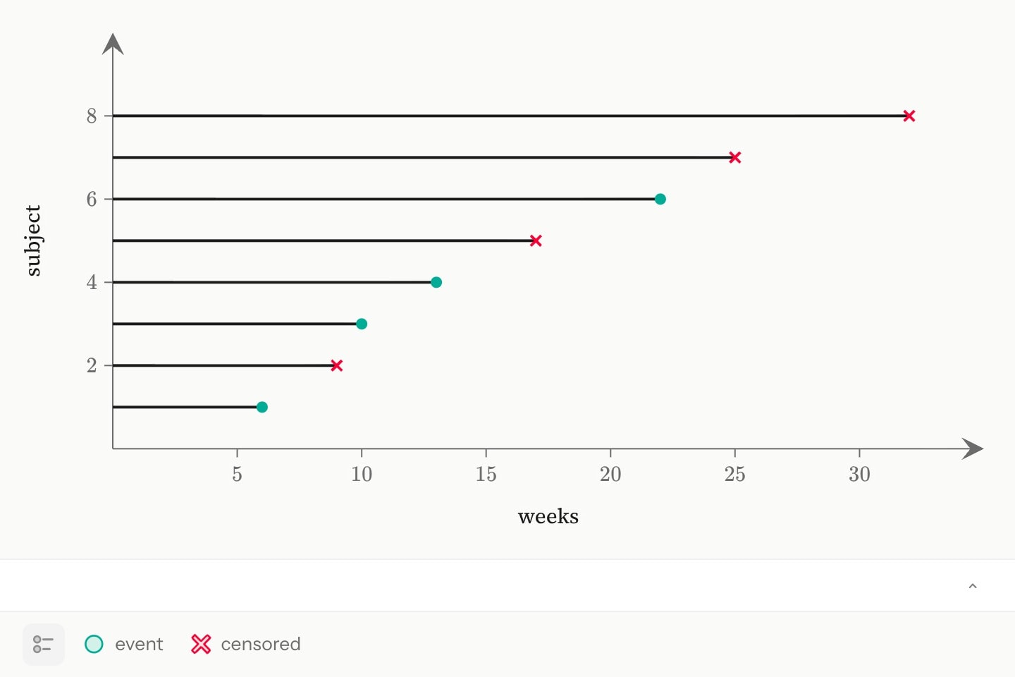
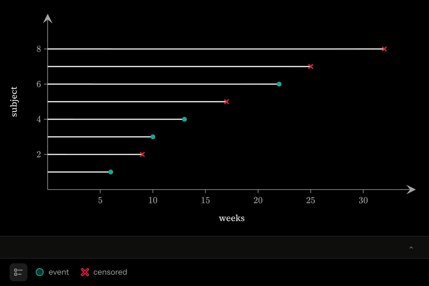
@data#trial{
    id | time | status
    1  | 6    | event
    2  | 9    | censored
    3  | 10   | event
    4  | 13   | event
    5  | 17   | censored
    6  | 22   | event
    7  | 25   | censored
    8  | 32   | censored
}

graph{
    @for(n: #trial; as: row){
        segment(start: (0, {{row.id}}); end: ({{row.time}}, {{row.id}}); colour: neutral)
    }
    scatter(
        x: #trial.time
        y: #trial.id
        colour: #trial.status -> event = teal, censored = red
        shape: #trial.status -> event = circle, censored = cross
    )
}(
    x axis label: weeks
    y axis label: subject
)

A shape map on a column of numbers is refused, since nothing lies between one shape and the next; band the numbers first.

scatter(x: #trial.time; y: #trial.id; shape: #trial.dose)

#Bands

Intervals as keys are bands, written as any interval is: [0, 25] holds both ends, [>0, <25] neither, and a missing end runs on for ever, [, 18.5] or [30, ]. An item takes the first band that holds its reading, so where two bands share an end the band written first has it. A reading no band holds is drawn in the mark's default colour.

The ends may be expressions of the scene's parameters, so a slider can move a threshold and the items change as it passes them:

Show code

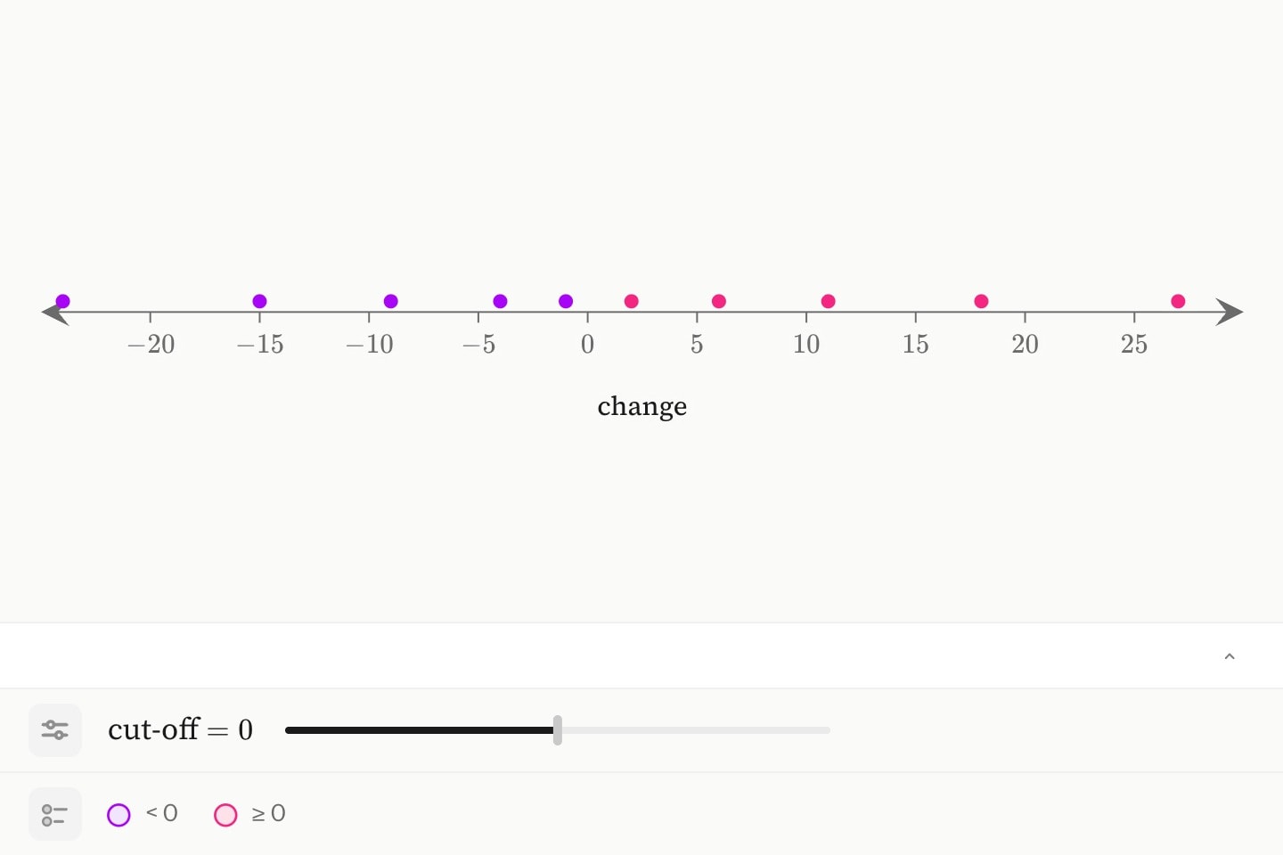
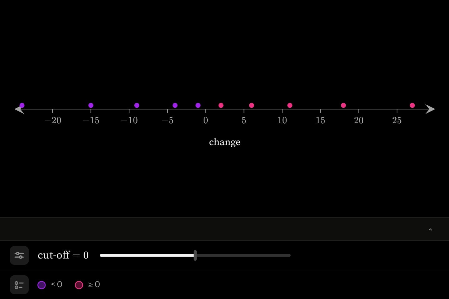
graph:x{
    slider:c(name: cut-off; range: [-20, 20]; step: 1; default: 0)
    scatter(
        x: -24, -15, -9, -4, -1, 2, 6, 11, 18, 27
        colour: value -> [, <c] = purple, [c, ] = pink
    )
}(
    x axis label: change
)

A column of names cannot be banded (canvas/channel-column), and a map's keys are all names or all intervals.

#Ramps

One interval mapped to a ramp name — multicolour, violet low to red high, or temperature, blue through white to red — is a ramp: each item's colour is its reading's place along the interval, the ends holding the readings past them. Below, the colour runs from 10 °C to 30 °C on the temperature ramp while the size follows population.

Show code

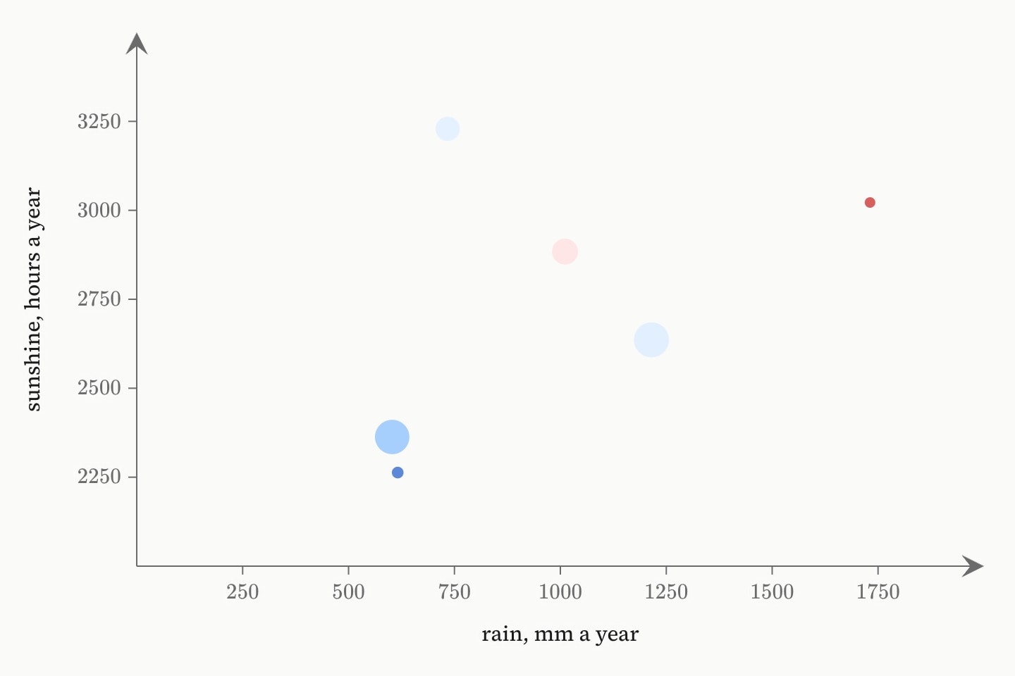
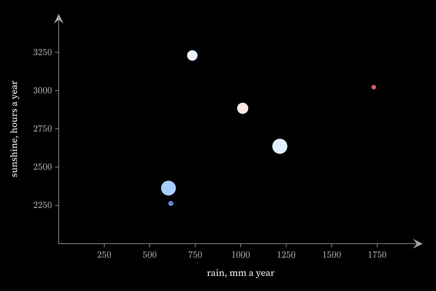
@data#cities{
    city      | rain | sun  | temp | people
    Hobart    | 616  | 2263 | 12.7 | 0.25
    Melbourne | 603  | 2363 | 15.9 | 5.2
    Sydney    | 1215 | 2636 | 18.6 | 5.4
    Perth     | 734  | 3229 | 18.8 | 2.3
    Brisbane  | 1011 | 2884 | 21.4 | 2.7
    Darwin    | 1731 | 3022 | 27.6 | 0.15
}

graph{
    scatter(
        x: #cities.rain
        y: #cities.sun
        colour: #cities.temp -> [10, 30] = temperature
        size: #cities.people -> [0, 6] = [4, 24]
    )
}(
    x axis label: rain, mm a year
    y axis label: sunshine, hours a year
)

A heatmap, surface, contour and field are coloured by their own values already, so their colour is the ramp or hue itself, and colour-domain gives the window it spans: heatmap(…; colour: temperature; colour-domain: [-1, 1]). A choropleth's values are the depth along its scale, and its colour-domain the window. Left out, the window is the least and greatest values drawn, and moves as they do.

#Sizes and widths

A column or a measurement alone draws AREA in proportion to the reading, so a reading twice another draws a mark of twice the area, the largest reading at the mark's largest size: size 20 on a scatter, size 12 on a marker, about two and a half times the plain radius on a vertex, and 6 pixels on an edge.

One interval mapped to another names the sizes instead: size: #cities.people -> [0, 6] = [4, 24] draws a reading of 0 at size 4 and 6 at size 24, area in proportion between them, and holds readings past the ends at the end sizes. Intervals mapped to one size each band the readings. The sizes are in the mark's own units — a scatter's and a marker's size, multiples of the plain vertex, and pixels of stroke for an edge's width.

Show code

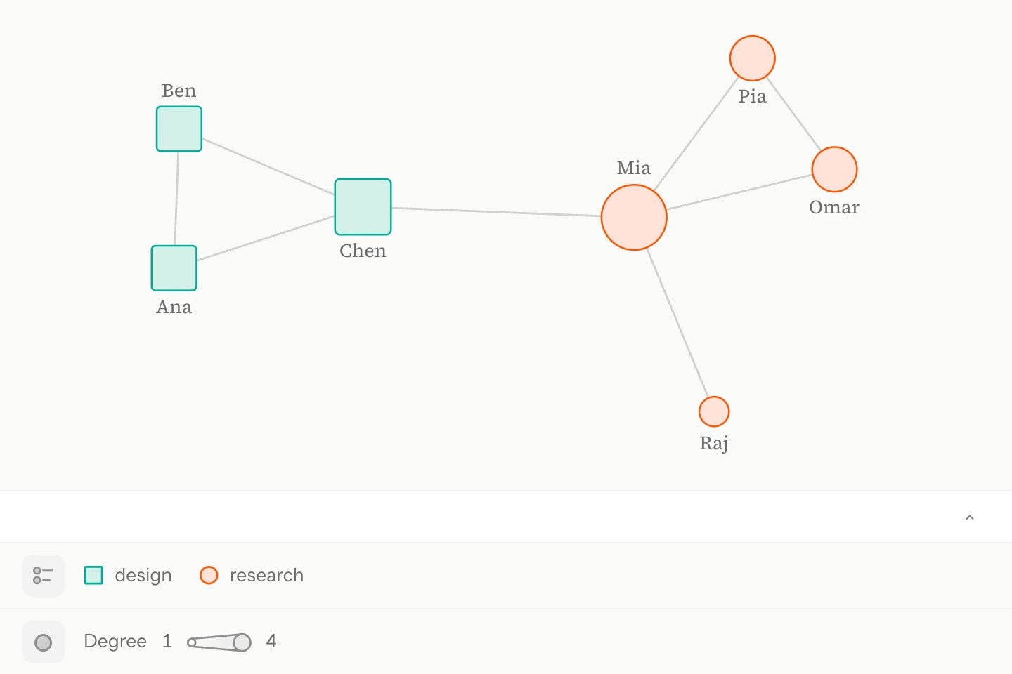
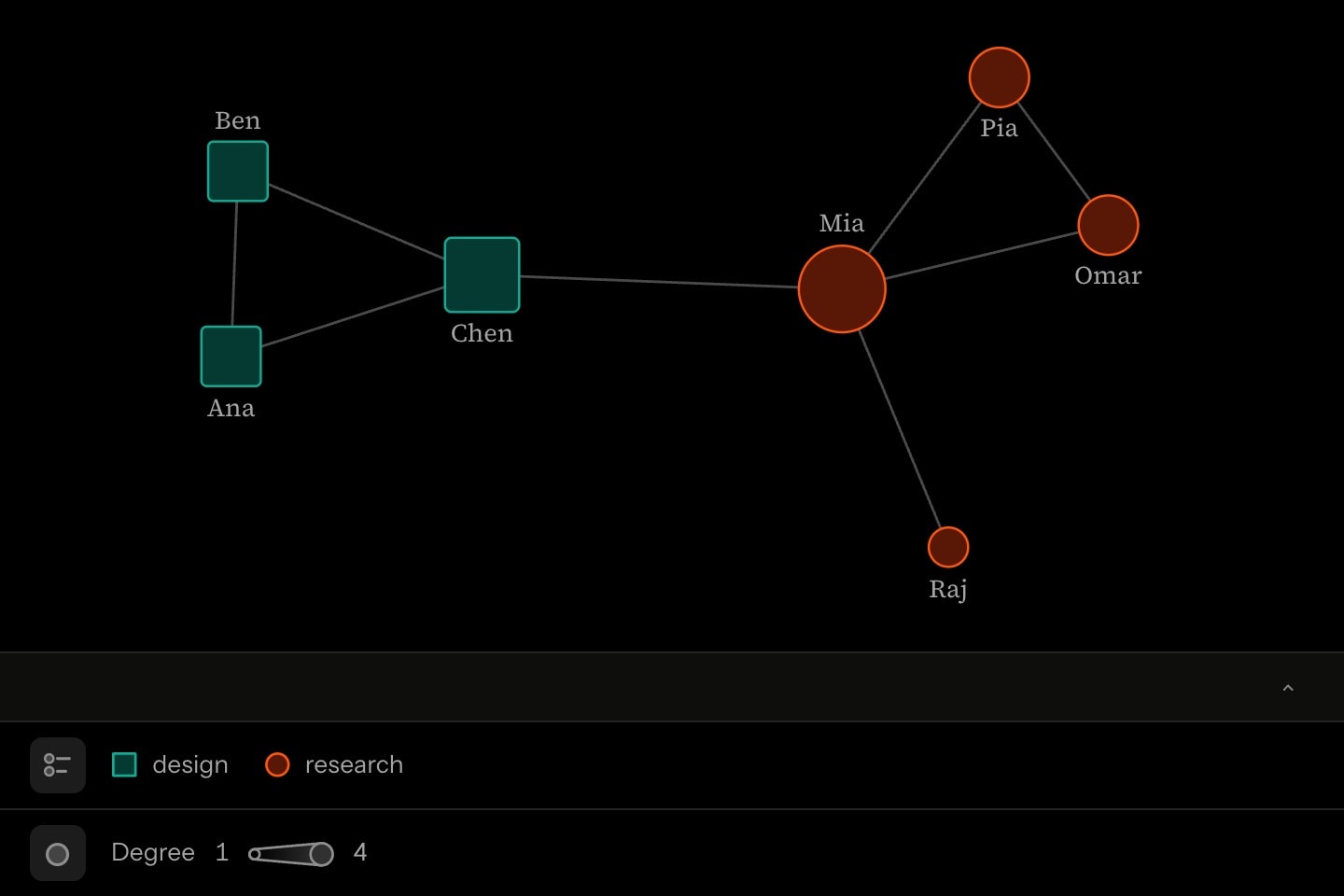
@data#people{
    name  | team
    Ana   | design
    Ben   | design
    Chen  | design
    Mia   | research
    Omar  | research
    Pia   | research
    Raj   | research
}

@data#ties{
    a    | b
    Ana  | Ben
    Ana  | Chen
    Ben  | Chen
    Chen | Mia
    Mia  | Omar
    Mia  | Pia
    Mia  | Raj
    Omar | Pia
}

network{
    vertices(
        names: #people.name
        groups: #people.team
        colour: group -> design = teal, research = orange
        shape: group -> design = square, research = circle
        size: degree -> [1, 4] = [1, 2.2]
    )
    edges(from: #ties.a; to: #ties.b)
}

#Which marks take which channels

• scatter: colour a constant, a list or a map; shape and size a constant or a map.
• bar, histogram and lollipop: colour a constant, a list or a map.
• heatmap, surface, contour and field: colour a ramp or a hue, with colour-domain.
• choropleth: colour one scale, a map from a column of categories to a scale each — every region shaded along its category's at the depth values gives it — or bands, every region flat in its band's colour; with colour-domain.
• marker: size a constant, or a map from a column.
• vertices: colour, size and shape, each a constant or a map.
• edges: colour and width, each a constant or a map.
• vertex and edge: constants, which win over whatever their table gives them.

In space (graph:xyz) a mark takes constants and lists, and a map is refused. A shape a mark does not draw is refused by name with the shapes it has: a vertex's are circle, square, diamond and none.

#The key, and group:

Every category and band a map draws is an entry in the scene's key, under its name or its interval: < 0, 0 – 25, ≥ 30. Where a colour map and a shape map follow the same driver, a name is one entry, its marker in its colour. A network's vertex size and edge width are scale rows from the least reading to the greatest, and the ramp of a heatmap, surface, field or choropleth is a scale row of its own. !legend on the environment turns the key off.

A map styles the items of one mark. group: on a mark, with the graph's key:, does a different job: it puts several marks under one entry, a colour or a stroke for each group — key: Projected = red dashed, Recorded = pink solid. What a mark's group pins wins over the mark's own colour, a map included.