fit
A least-squares fit through the observations of the scatter named in of:, and no others — a graph may carry two fits over two scatters. model chooses the family and degree the polynomial degree; giving degree a parameter rather than a number puts the degree under the reader's control through that parameter's slider. Publishes derived slope, intercept and r2.
fitxyplane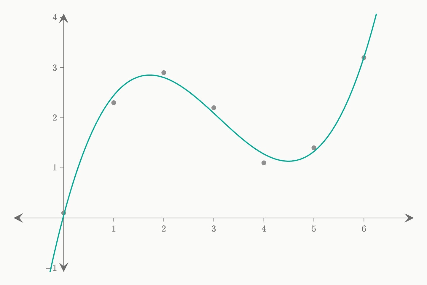
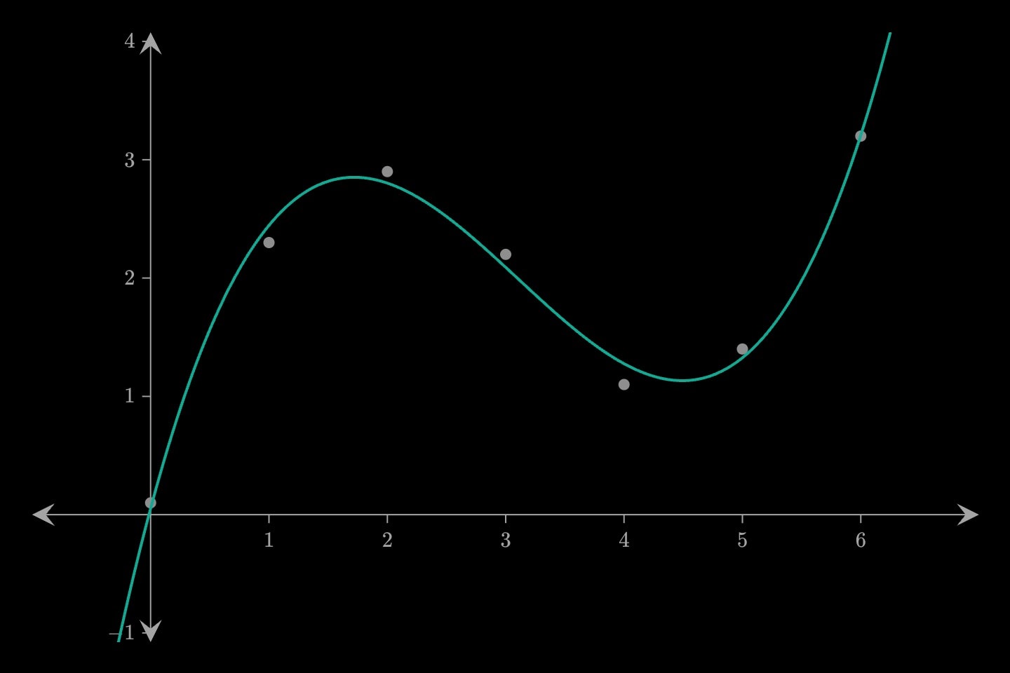
A fit is the least-squares line or polynomial through one scatter's observations, named in of: — its head slot, so fit: #observations is the same as fit(of: #observations). Give degree a parameter instead of a number and the reader drives it — Interaction shows that pairing. residuals draws the differences from a fit to the points it was found from.
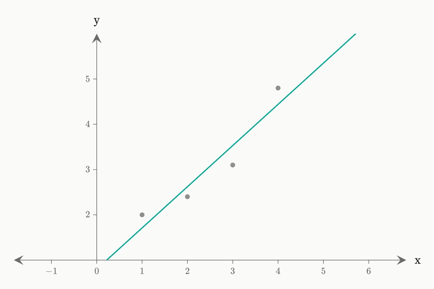
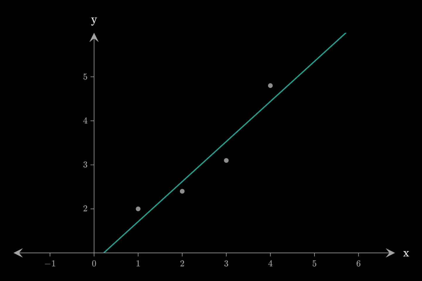
canvas.graph#fit-graph{
    scatter#observations(x: 1, 2, 3, 4; y: 2.0, 2.4, 3.1, 4.8; colour: grey)
    fit(of: #observations; model: polynomial; degree: 1; colour: teal)
}(
    x-axis-label: x
    y-axis-label: y
)
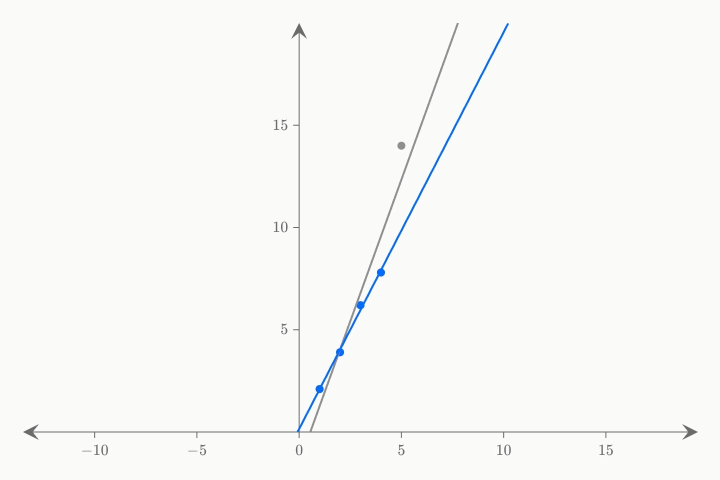
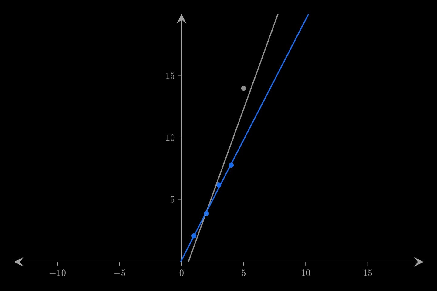
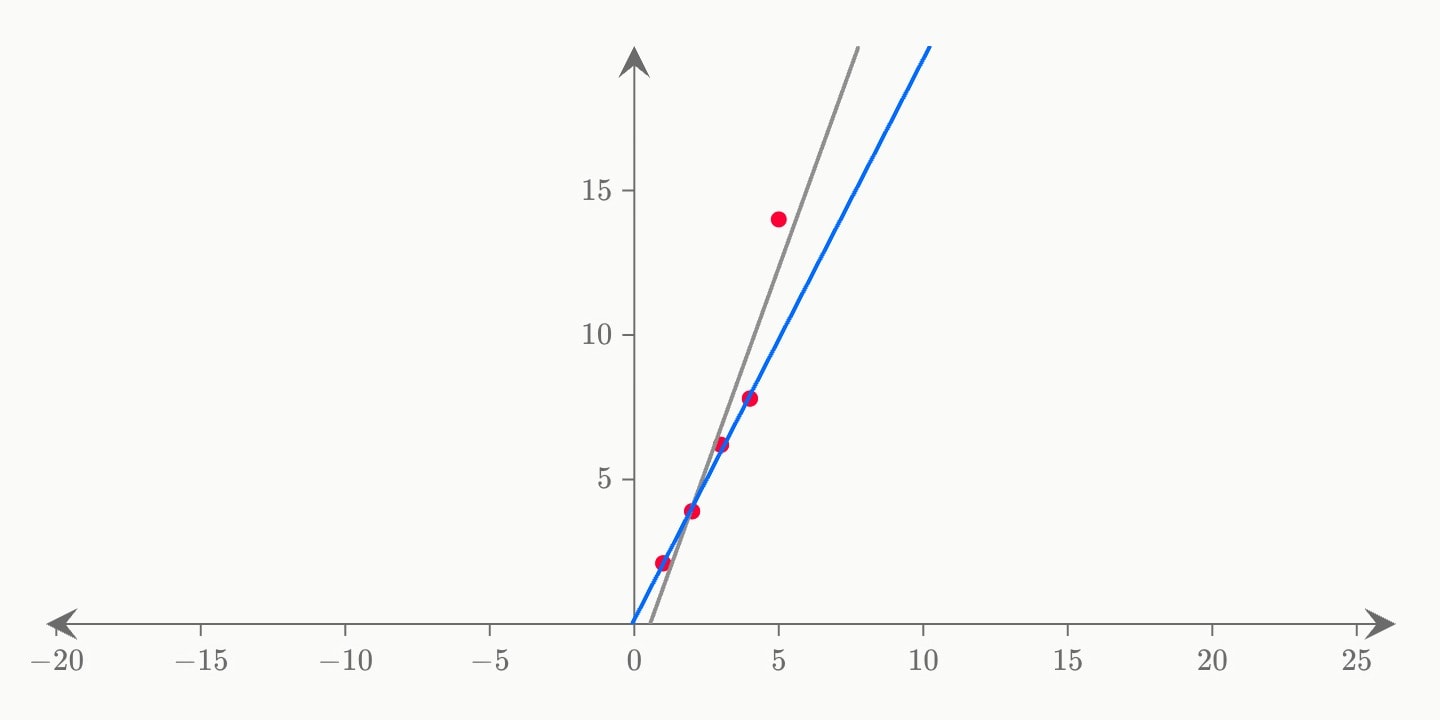
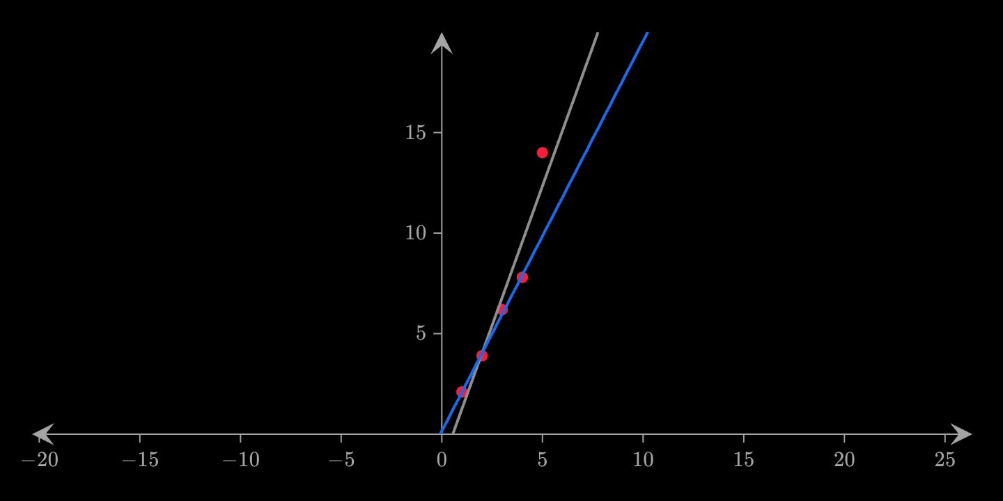
A fit fits the mark it names and nothing else, so a graph can carry two of them: draw the sample twice, once whole and once without the point in question, and the two lines stand beside each other with their own slope and r2. To fit part of a sample, draw that part as its own scatter and fit that.
canvas.graph{
    scatter#all(x: 1, 2, 3, 4, 5; y: 2.1, 3.9, 6.2, 7.8, 14.0; colour: grey)
    scatter#typical(x: 1, 2, 3, 4; y: 2.1, 3.9, 6.2, 7.8; colour: blue)

    fit#with-outlier(of: #all; degree: 1; colour: grey)
    fit#without(of: #typical; degree: 1; colour: blue)
}slope, intercept and r2. The slope is the fitted polynomial's derivative at zero — exact, and live under whatever degree is in force — so prose citing {{#f.slope}} cannot disagree with the graph.#Attributes
offit(of: #readings). The fit is taken through that mark's observations alone, so two scatters in one graph carry two independent fits. To fit part of a sample, draw that part as its own scatter and name it here.through, dataCan be written as shorthand: fit:valuemodelpolynomiallinearpolynomialdegree1colourbluelight-bluedark-blueredlight-reddark-redorangelight-orangedark-orangeyellowlight-yellowdark-yellowteallight-tealdark-tealgreenlight-greendark-greenpinklight-pinkdark-pinkpurplelight-purpledark-purplegreylight-greydark-greyneutralhex(…)rgb(…)colortealwidth2hiddenhidden: true !cue.to{false}(at: 2) reveals it — and unlike a cue, a hidden element still frames the plot, so the axes do not jump when it appears.falselockeditable: graph. Nothing at all on a graph that is not editable.lockedfalse#Derived attributes
Computed while the element renders — read one with #id.name in attribute position or {{#id.name}} in prose, never set.
slopeinterceptr2#Allowed in
#Examples
canvas.graph{
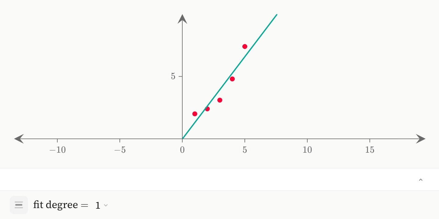
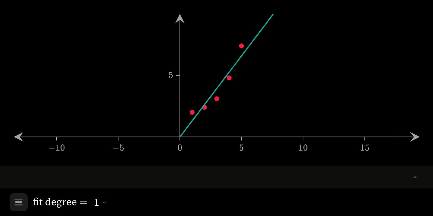
    scatter#readings(x: 1, 2, 3, 4, 5; y: 2.0, 2.4, 3.1, 4.8, 7.4)
    selector:d(name: fit degree; options: [1, 2, 3, 4])
    fit(of: #readings; model: polynomial; degree: d; colour: teal)
}
canvas.graph{
    scatter#all(x: #trial.dose; y: #trial.response)
    scatter#typical(x: #clean.dose; y: #clean.response)

    fit#with-outlier(of: #all; degree: 1; colour: grey)
    fit#without(of: #typical; degree: 1; colour: blue)
}