field
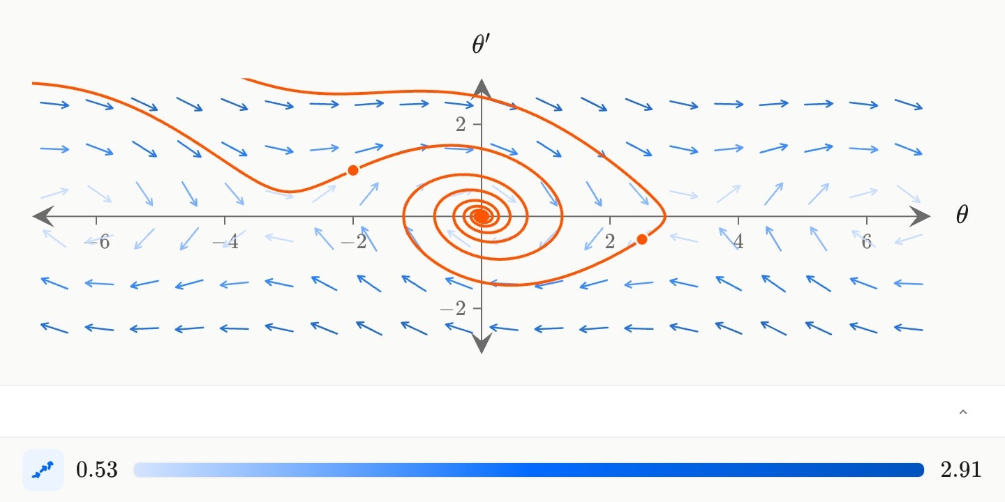
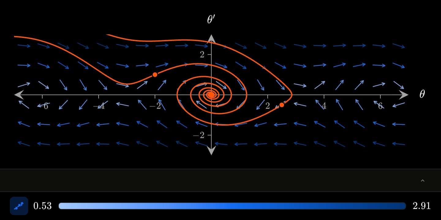
A differential equation drawn as the directions it gives, and the solutions that follow them. field: x - y is a first-order equation , drawn as a slope field of headless ticks; field(dx: y; dy: -x) is a system , drawn as a direction field of arrows — the phase plane. On the argand plane the one expression is and the field is the flow of . Every arrow is the same length; the field's strength is its colour. Seeds in from: are integrated forward and back until the solution leaves the window, comes to rest or closes a loop, and the reader may drag them. x and y are the axes here, not parameters: only the letters beyond them get footer sliders.
fieldxyargandplane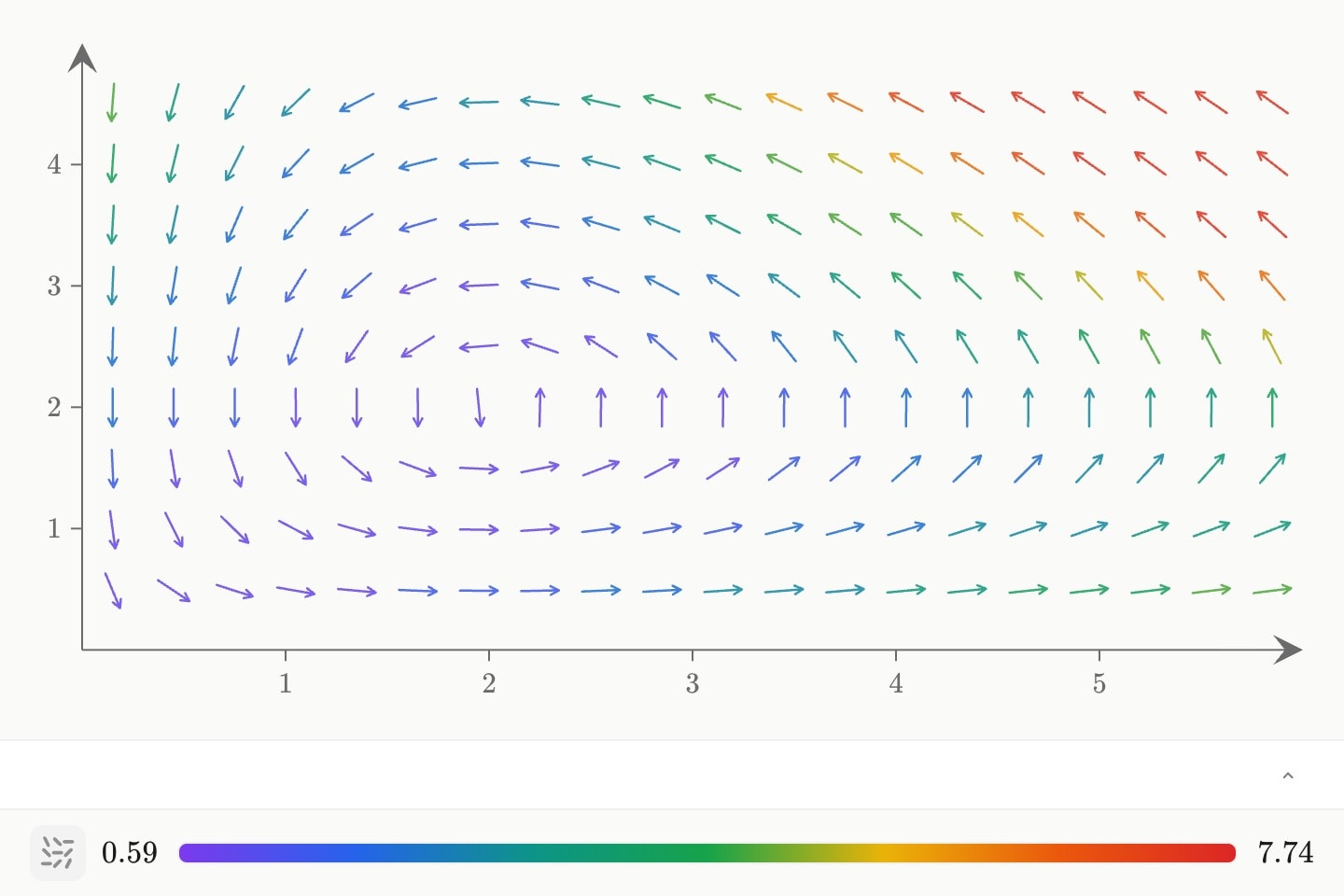
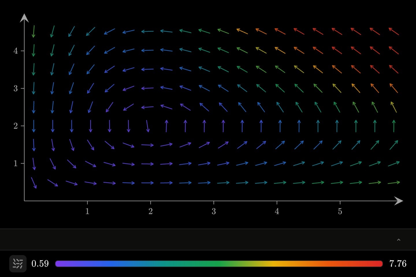
A field draws a differential equation: at each point of a grid, an arrow in the direction the equation gives there. Every arrow is the same length, so the direction is what you read, and the field's strength is its colour — a colour that is a single hue or a ramp, as a contour's is. The footer carries the key and reads off the strength under the cursor. density sets how many arrows run across the plot, 20 unless you say otherwise.
#Slopes and systems
field: x - y is a first-order equation, y′ = x − y. It is drawn as a slope field: short ticks without heads, since a slope has a steepness but no forward, and coloured by how steep it is. field(dx: y; dy: -x) is a system of two, x′ and y′, drawn as arrows. This is the phase plane, where every point is a state and the arrow says where the state goes next. Write one form or the other; both together are refused.
On the argand plane a field is one function of z: field: z^2 - 1 draws the flow of z′ = f(z), with the arrow at z pointing along f(z). The number line and the polar plane take no field.
x and y are the axes in a field's expressions, not parameters. Any other letter is a parameter, r included: dy: r * y * (1 - y) is logistic growth with a slider for its rate.#Solutions
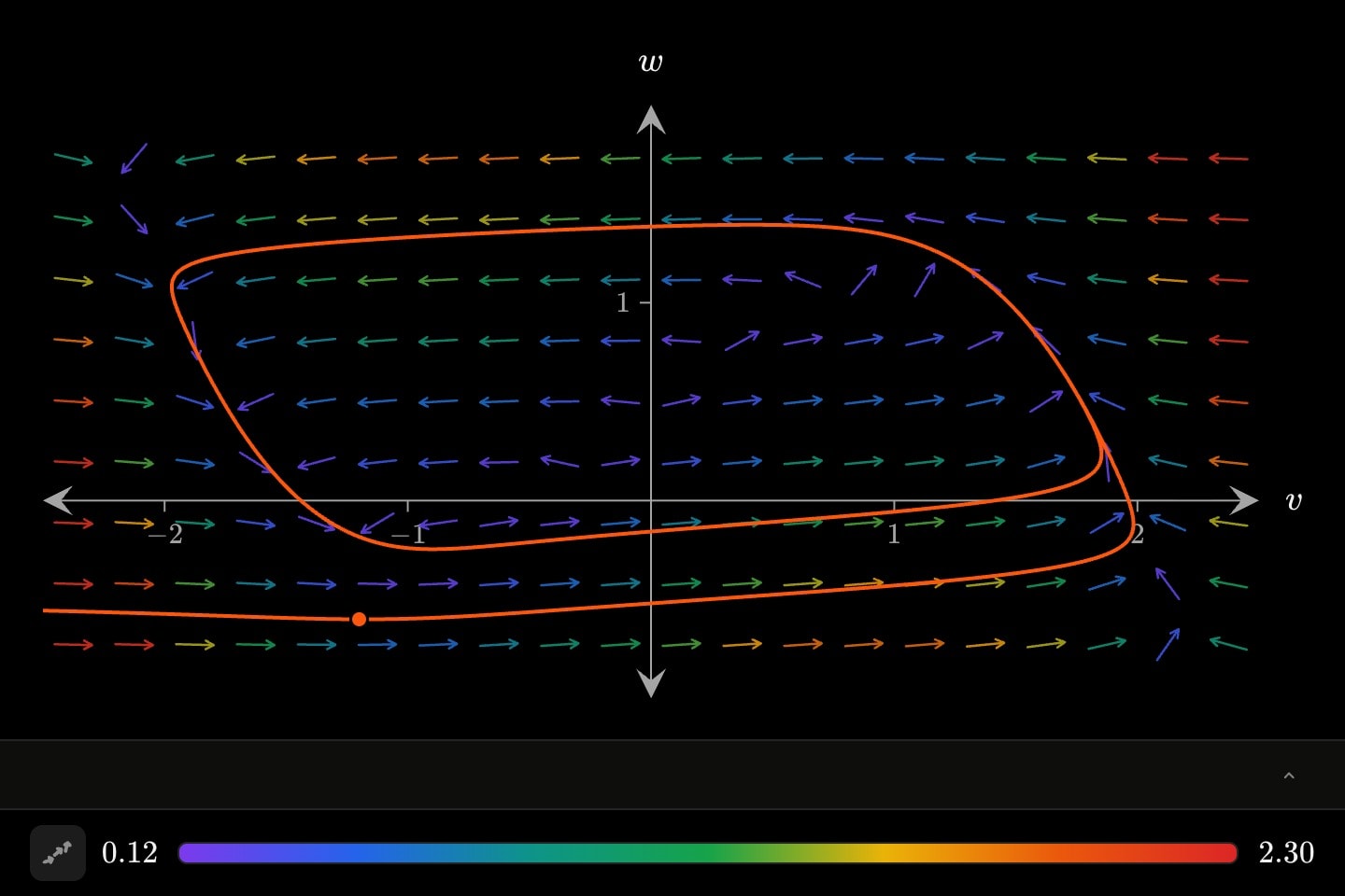
from starts solutions at points of the plane: from: (1, 0), (2.5, 0). Each is followed both ways in time until it leaves the window, comes to rest or closes a loop, and it is worked out again whenever a parameter moves. span: [0, 5] runs it over that stretch of time instead, forward only. The reader can drag a starting point, and the solution through it follows; draggable: false fixes them. arrows: false leaves only the solutions. solution-colour and solution-width style them.
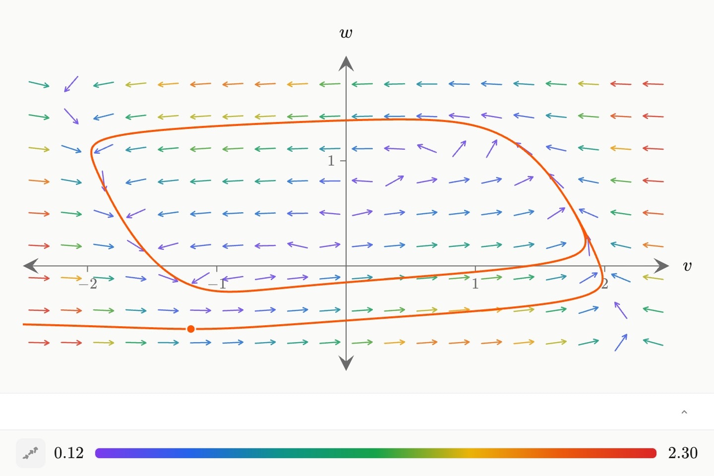
canvas.graph{
    field(
        dx: x - x^3 / 3 - y + 0.5
        dy: 0.08 * (x + 0.7 - 0.8 * y)
        from: (-1.2, -0.6)
    )
}(
    x-domain: [-2.5, 2.5]
    y-domain: [-1, 2]
    x-axis-label: $v$
    y-axis-label: $w$
)#Drawing, tracing and flow
Inside a cue.draw, each solution is drawn in from its earliest time to its latest while the arrows fade in. A cue.trace can name the field as its path, path: #phase, and rides the first solution at the same pace, so a dot and the line it draws arrive together. flow: true sets dots moving along the field at its own speeds: they crawl where it is weak and race where it is strong. They stay still for a reader who has asked for reduced motion.
#Attributes
expressiondx and dy, never beside them.field-expressionslope, f, exp, func, functionCan be written as shorthand: field:valuefromfrom: (1, 0), (2.5, 0). A cue.trace naming the field rides the first one.seeds, throughspan[0, 5] runs forward only. Absent, a solution runs both ways until it leaves the window, comes to rest or closes a loop.t, timedensity20arrowstrueflowfalsedraggabledragtruecolourblueredorangeyellowtealgreenpinkpurplegreyhex(…)rgb(…)multicolourtemperaturecolormulticolourwidth1.25opacity0.85solution-colourbluelight-bluedark-blueredlight-reddark-redorangelight-orangedark-orangeyellowlight-yellowdark-yellowteallight-tealdark-tealgreenlight-greendark-greenpinklight-pinkdark-pinkpurplelight-purpledark-purplegreylight-greydark-greyneutralhex(…)rgb(…)solution-colororangesolution-width2hiddenhidden: true !cue.to{false}(at: 2) is its reveal.falselocklockedfalselayerxyplanedxdy.field-componentdydx.field-component#Examples
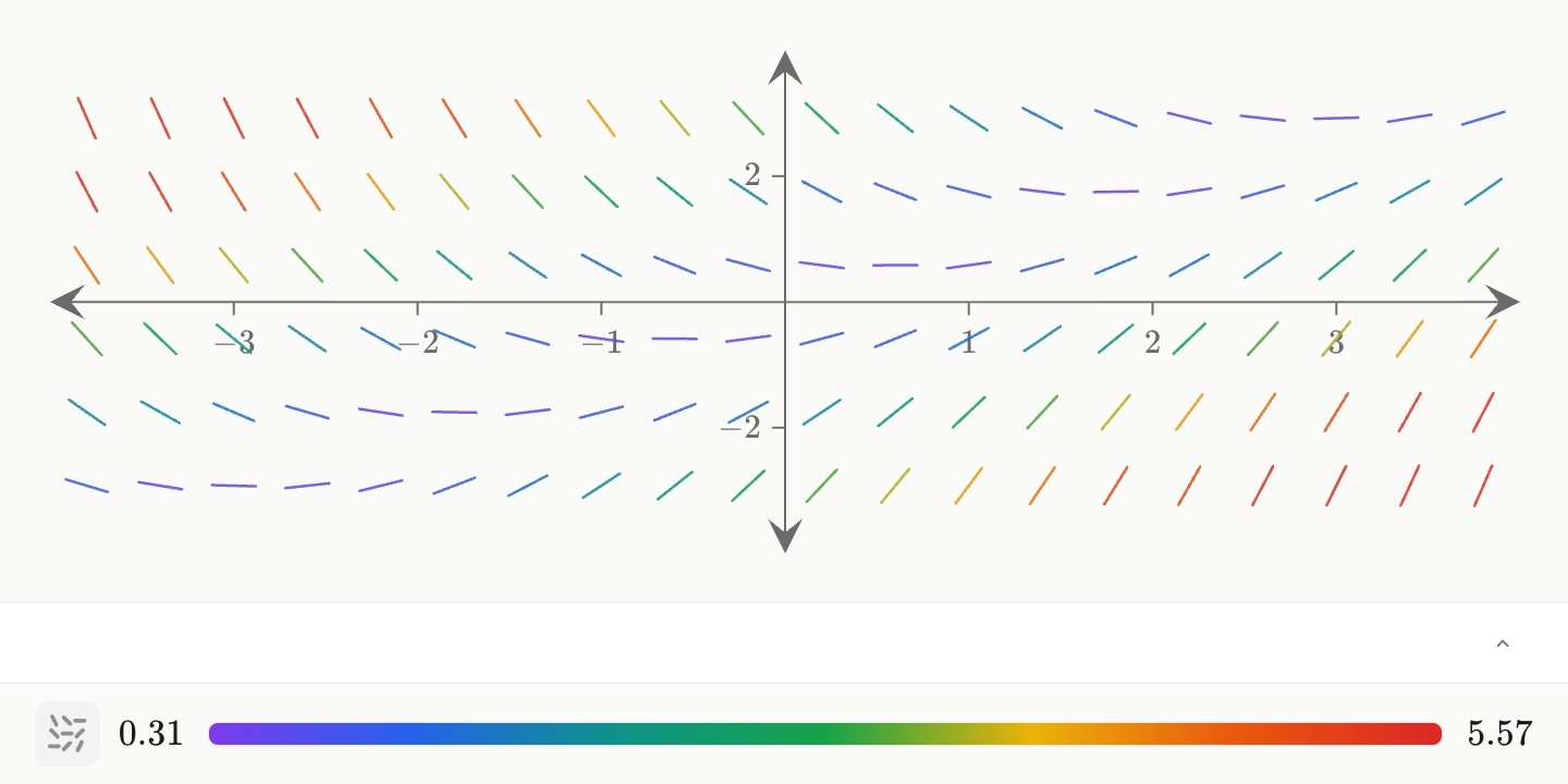
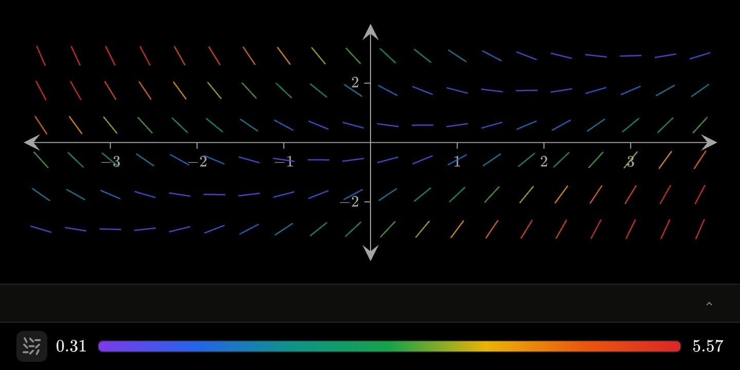
canvas.graph{
    field(slope: x - y)
}(
    x-domain: [-4, 4]
    y-domain: [-4, 4]
)
canvas.graph{
    field(
        dx: y
        dy: -sin(x) - 0.3 * y
        from: (-2, 1), (2.5, -0.5)
        colour: blue
    )
}(
    x-domain: [-7, 7]
    y-domain: [-3, 3]
    x-axis-label: $\theta$
    y-axis-label: $\theta'$
)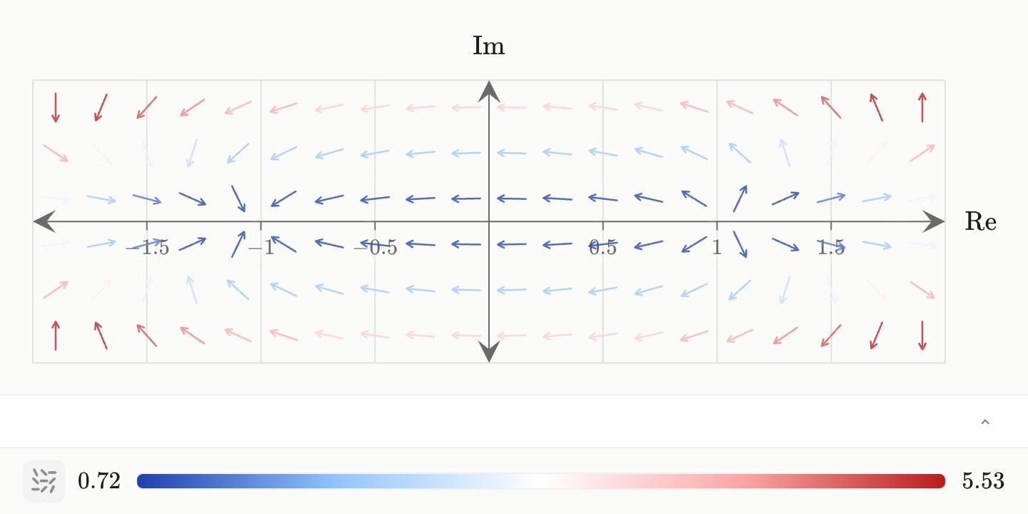
canvas.graph:argand{
    field(f: z^2 - 1; colour: temperature)
}(
    re-domain: [-2, 2]
    im-domain: [-2, 2]
)