graph
A plotting environment on the scene's canvas. Its body holds marks — scatter, curve, line, the shapes, fit and the surfaces — and the parameters that drive them, each of which gets a slider in the environment footer. It draws its own frame, and the x and y domains are animatable with !cue.to.
graph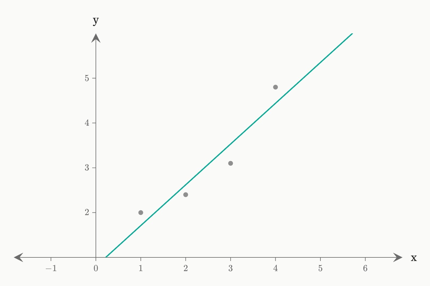
#The graph environment
graph is a plotting surface: its body holds marks, it draws its own frame, and its domains are animatable. It carries the environment's id — graph#projectile{...} — and the frame is set by x-domain / y-domain (derived from the data when omitted), x-axis-label / y-axis-label, show-grid, show-axes, show-ticks, and show-background as the master switch. show-ticks: false hides the axis's own numbers and nothing else — axis.label names stay, and the gutter shrinks to what is left in it.
Two more the frame carries. aspect: square takes the largest square the margins leave and centres the plot in it — a square frame, not a square unit. Leaving both domains off already gives a picture whose x unit and y unit are the same length on screen, which is right where both axes carry the same thing and wrong where they do not: a quantile-quantile plot is read by whether its points lie along the 45° line, and only a square frame makes that fair, while its two axes are a sample against a distribution and must keep their own scales. Under aspect: square they do, and the two never share a grid step. And seed is the one number every settled pseudo-random thing the graph draws comes from — today the offsets of a scatter(layout: jitter). Which noise a jitter uses is arbitrary; that it is the same noise on every render, in every browser and in three years is not, so the offsets are a function of the seed and the reading's own row and of nothing else. Change the seed and the same sample is arranged differently, which is how a cloud that happens to hide a point is fixed without touching the data.
#Planes
A graph's head names its plane — what a coordinate on its marks is. graph:xy is the ordinary plane and the default; graph:x a number line, with one axis and marks that take x alone; graph:argand the complex plane, whose axes are re and im and whose marks take one complex z — point(z: 3 + 2i), point(z: (3 + 2i)^2), with i a constant and every expression complex-valued — or re and im apart, which is how two columns bind; graph:polar, whose axes are r and theta, the angle in radians unless written 60deg. A pair — a segment's ends, an angle's corner — is (a, b) on every plane, read in the plane's own axes.
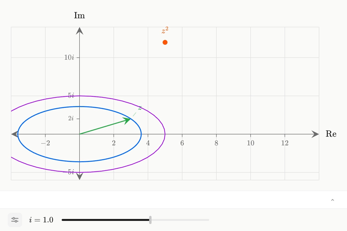
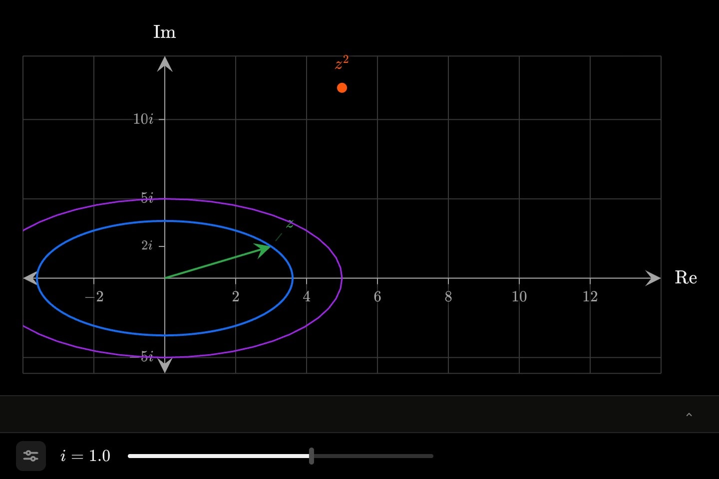
graph:argand{
    vector(z: 3 + 2i; label: $z$)
    point(z: (3 + 2i)^2; label: $z^2$)
    circle(z: 0; size: abs(3 + 2i); fill: false)
    curve(z: sqrt(13) * e^(i * t); t: [0, 2pi])
    axis.label(im: 2; label: $2i$)
}(
    re domain: [-4, 14]
    im domain: [-6, 14]
)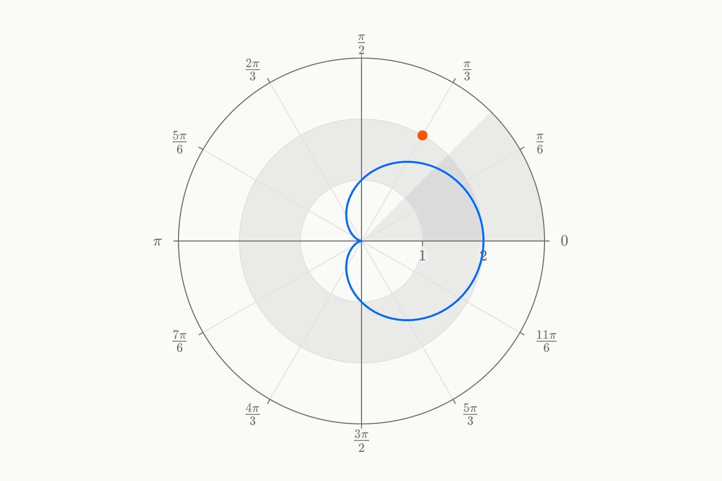
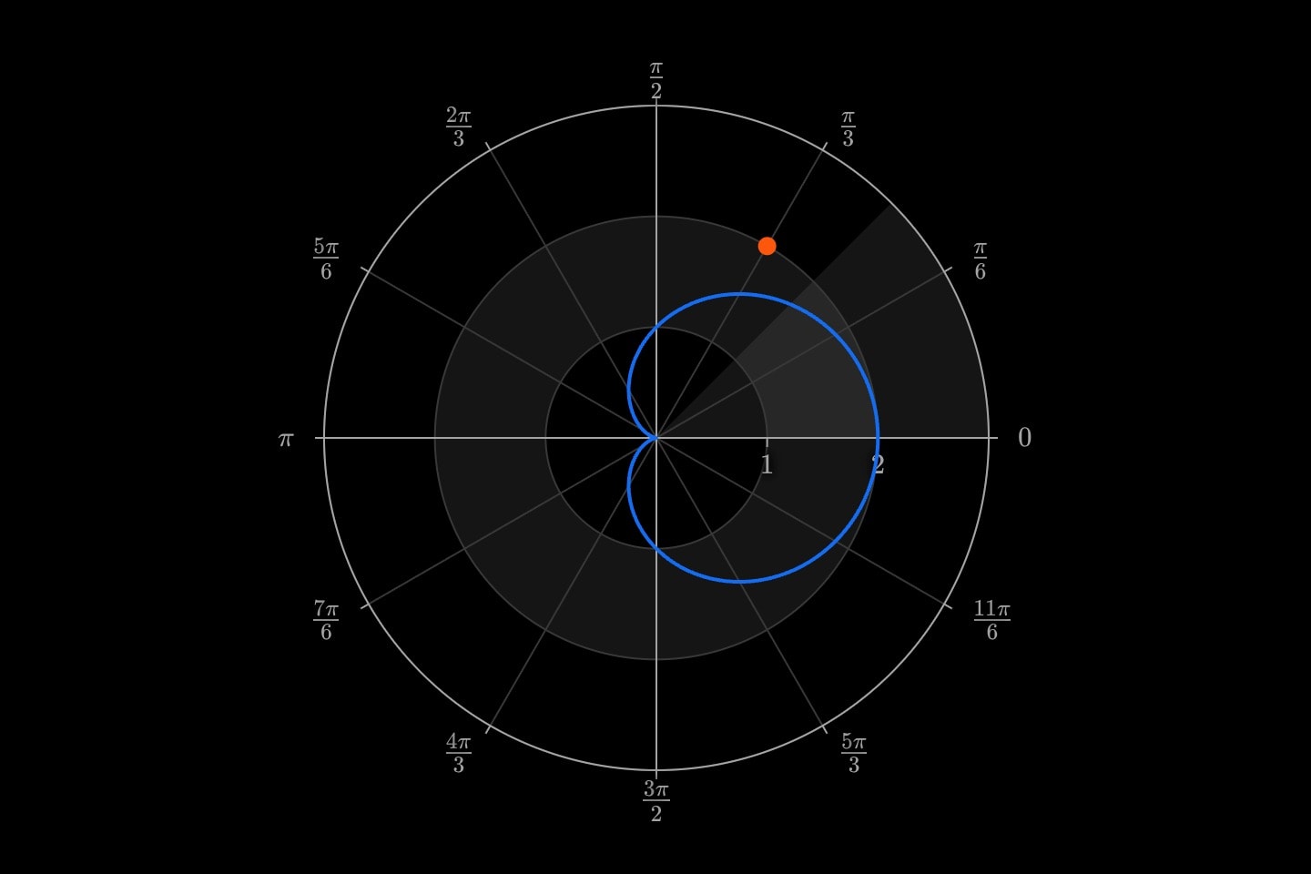
graph:polar{
    curve(expression: 1 + cos(theta))
    point(r: 2; theta: 60deg)
    axis.band(r: [1, 2])
    axis.band(theta: [0, pi/4])
}(
    r domain: [0, 3]
)
A plane admits the marks it can draw and nothing else — the compiler says which when one is refused, and why. The argand plane has no independent axis, so fit, integral and curve: f are not drawn there (a curve on it is z(t)); the polar plane refuses integral, whose area is not the one it computes; the number line draws positions and series and nothing that needs a second axis. Each mark's page says where it is drawn. The same rules hold for a mark inside a cue. Every plane's axis attributes are spelled with the axis's name in front — re domain:, r domain:, theta format: — and the other planes' are refused.
#Axes
An axis has two properties, written with its name in front and combining with each other and with any plane. x format: is what the axis holds: numbers; radians, which sets each label as a fraction of π and rules the axis in π — its automatic grid step comes off the π ladder, π/4, π/2, π, 2π; degrees, whose values are still radians and whose labels read 30°; dates, which places 2024, 2024-03, 2024-03-15 and a date column at their fractional years and ticks by span; the preset series months and weekdays (ticks Jan…, Mon…); and a written list — x format: Red, Blue, Yellow — or a dataset column — x format: #sales.region, its distinct cells in row order. A series makes the axis categorical: the names stand at positions 1…n, every mark on the axis speaks them (line(x: Mon, Tue, Wed; y: 12, 19, 15)), a column of names binds directly, and a name the axis does not have is a compile error. A continuous mark — curve, fit, integral — is refused on a categorical axis: there is nothing between two names to draw it over.
#Axes ruled in discrete numbers
x format: discrete is the same axis in numbers. The values its marks give are sorted, de-duplicated, and stood at 1…n one apiece: five loads of 2, 3, 4, 5 and 6 kN get five stops, and so do four speeds of 800, 1200, 1600 and 2000 rpm. The stops are evenly spaced however far apart the numbers themselves are, each tick writes the value it stands for, and there is nothing between two stops — no tick at a round thousand that falls between two of the speeds actually run, and no room for a reading nobody took.
That is the right axis whenever the numbers are settings rather than measurements: the levels of a factorial experiment, a die's six faces, the years a census was taken. It is the wrong one when the gaps carry meaning — bins of unequal width, readings at irregular times — because it throws the spacing away. numbers is the axis for those, and the difference is worth deciding rather than inheriting: a value the axis was not ruled at is a compile error on a discrete axis, exactly as an unknown name is on a categorical one.
auto, the default, is decided from the marks: a categorical series on the axis rules it in those names, in the order they first appear; a date column or literal rules it in dates; an axis carrying nothing but heatmap cells rules itself discrete at their values, since a cell exists at its own setting and nowhere else; otherwise the axis holds numbers. Write the values out when the order or the full set matters — a Likert scale, a category with no data that must still appear.
x scale: is how the axis places a value: linear, log (v at log₁₀ v) or log2. A transform, not a relabelling — the data is written as measured, scatter(x: 10, 100, 1000), and the axis puts each reading at its logarithm: curves are sampled in it, a fit on log–log gives the exponent as its slope, domains and !cue.zoom windows stay in data units, and the ticks are the decades written as values. A literal at or below zero is a compile error; a cell at or below zero drops its row. A scale beside names, dates or angles is refused, and it is never auto.
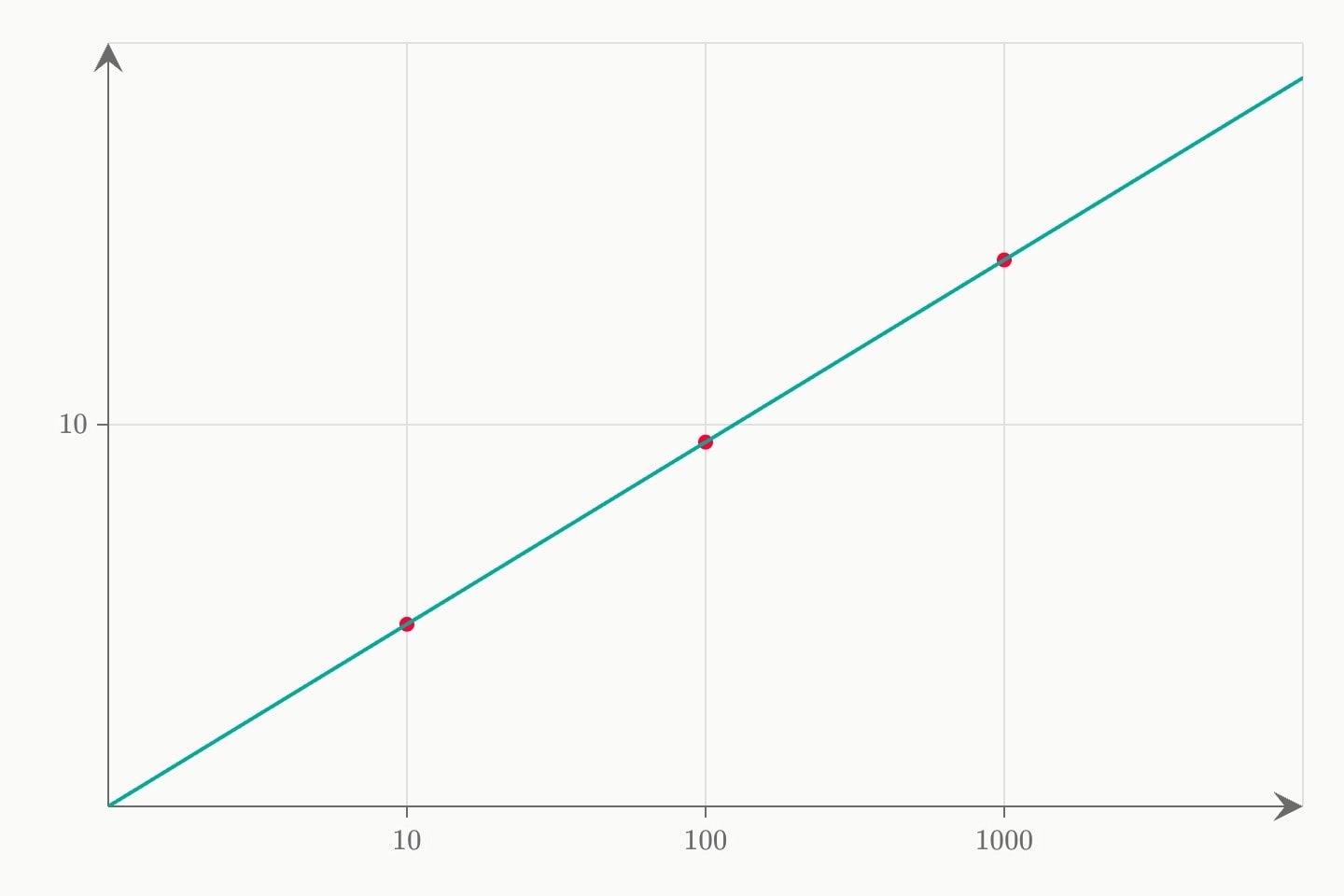
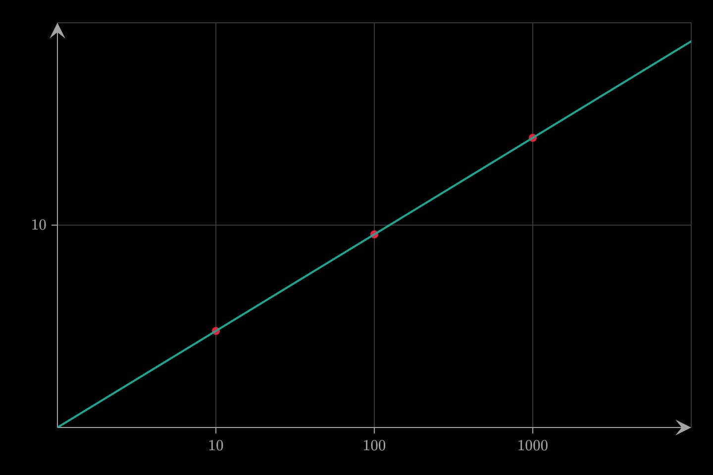
graph{
    scatter#readings(x: 10, 100, 1000; y: 3, 9, 27)
    fit(of: #readings; degree: 1)
}(
    x scale: log
    y scale: log
)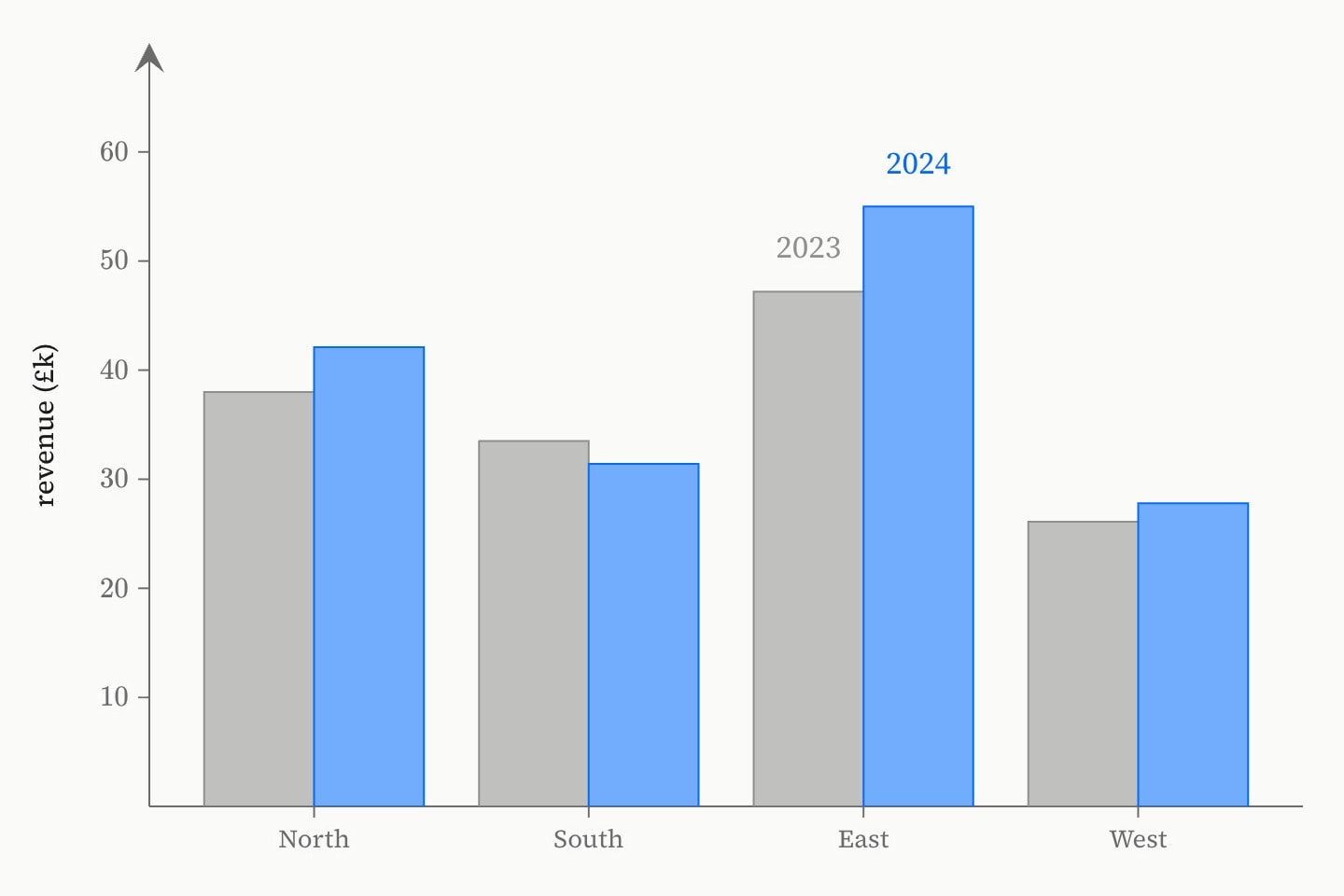
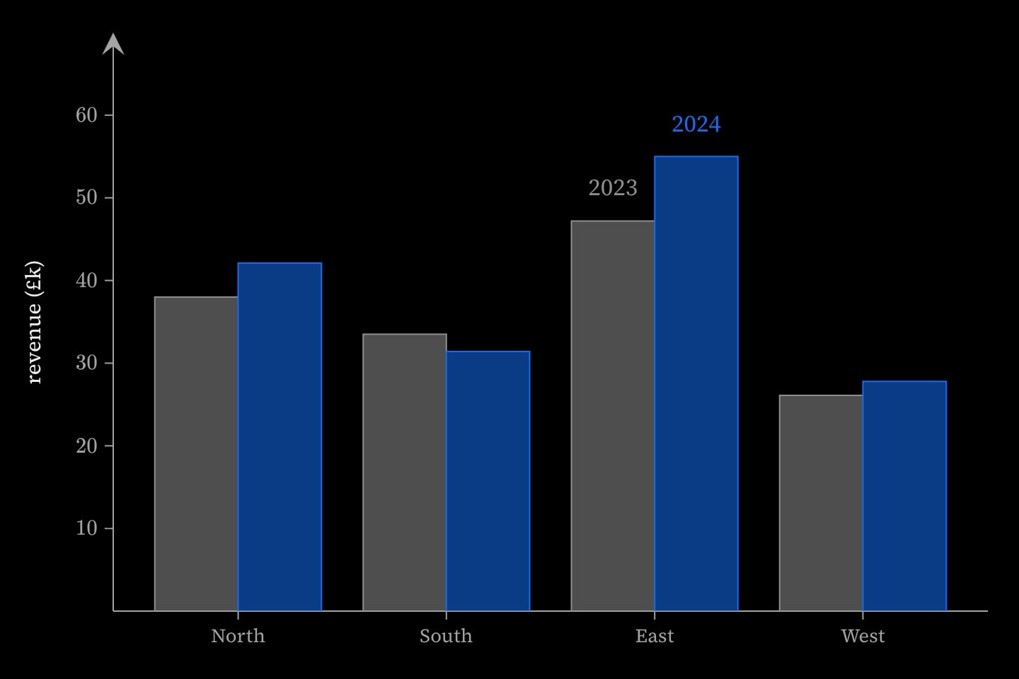
graph{
    @data#sales{
        region | y2023 | y2024
        North  | 38.0  | 42.1
        South  | 33.5  | 31.4
        East   | 47.2  | 55.0
        West   | 26.1  | 27.8
    }

    bar(x: #sales.region; y: #sales.y2023; colour: grey; label: 2023)
    bar(x: #sales.region; y: #sales.y2024; colour: blue; label: 2024)
}(
    y axis label: revenue (£k)
)#Marks
Everything drawn on the surface is a mark, and marks share a set of attributes: colour, label (rich text, so $maths$ sets properly), hidden (declared but not drawn — and animatable), lock (protects the mark on an editable: graph), and layer (paint order). Every outline takes dashed, which is how a figure draws the shape that is not there. Each mark's own page opens with what it draws and how to write it; by what they draw, they are:
- Positions and figures —
point,line,segment,vector,polygon, and theshapes, which differ only in outline. - Notation —
anglemarks and measures the angle at a vertex,bracespans a distance and names it, andtextsets words anywhere in the picture. - Functions —
curveplots an expression or a position int;integralshades the area under one;contourandsurfacedraw a function ofxandy, traced and shaded;fielddraws a differential equation as arrows, with the solutions through chosen points. - Readings —
scatterandlollipopdraw readings at positions,barstands one at each name, andhistogrambins a sample on a numeric axis;heatmaplays a value out in a grid of cells, which is what a correlation matrix is. Every one binds a dataset column directly; thepage covers where columns come from. - Summaries of a sample —
boxplot,violinanddensitytake the readings themselves and work the summary out. - Models —
fitlays a least-squares line or polynomial through a scatter, andresidualsdraws each reading's distance from it. - Axis annotations —
axis.labelnames a value on an axis,axis.bracenames an interval beside it,axis.bandshades one across the plot, andaxis.breakcuts one out of the axis.
#Where marks stand
Some marks draw a sample rather than a position, and those stand. On the number line a scatter, a boxplot and a violin each take a lane above the line, in source order, the first sitting on the line.
On a plane a mark stands at a place on the other axis. Written with one coordinate — x: and it lies along the x axis, y: and it stands up the y axis — its on: says where. A number there stands it at that value; a name stands it at that name and rules the axis in the names its marks stand at, so three samples side by side need no x format: line. The room at a place is the band there — a unit on an axis of names, and on a continuous one the closest two places stand, so nothing at one can overlap anything at another. Everything standing at one place splits that room in source order, as several bar marks split the band at one name; width: is each mark's share of its slot.
graph:xy{
    boxplot(y: #trial.control; on: control; colour: blue)
    scatter(y: #trial.control; on: control; colour: grey)
    boxplot(y: #trial.treated; on: treated; colour: orange)
    scatter(y: #trial.treated; on: treated; colour: grey)
}(
    y axis label: mass (g)
)
A box, a violin and a scatter of the same readings are one sample drawn several ways, and share one lane or slot rather than splitting it: the summary lands over the readings with nothing to position by hand, and which is drawn over which is source order and layer. Written with both coordinates and one axis ruled in names, a mark stands at every name at once, each reading at the name in its own row — the shape data usually arrives in, one row per reading and a column saying which group it belongs to. The names are drawn at the edge of the plot whatever the other axis's window holds: an axis ruled in names never crosses at the origin, so a diverging plot centred on zero keeps its names clear of the marks.
#Derived attributes
Marks that compute something publish it for reading: a curve's max and min, a fit's slope, intercept and r2, an integral's value, a surface's min and max, a boxplot's median, q1, q3, iqr, min and max (under each axis's name where it summarises a pair of samples), a parameter's value. Reach one by member access on the mark's id — #f.slope in an attribute, {{#f.slope}} in prose. Derived attributes covers how they behave.
#Attributes
planex a number line, xy the ordinary plane (the default), argand the complex plane (re/im, or one complex z), polar (r/theta). The head form — graph:polar{…}. A plane admits the marks it can draw and withdraws the other planes' axis attributes; a mark inside a cue is held to it just the same.graph:valuexytitle$maths$ and inline formatting render. A named attribute: the head : names the plane.editablefalseinteractivefalseshow-tickstickstrueshow-axesaxestrueshow-backgroundbackground, show-bg, bgtrueshow-gridgridtruegrid-styleof: 'lines' is squared paper, 'dots' steps back and lets the marks carry the picture. The -minor variants add unlabelled subdivisions between the labelled lines.lineslines-minordotsdots-minorgrid-typelinesseedscatter(layout: jitter). Which noise a jitter uses is arbitrary; that it is the same noise every time is not, since a picture that rearranged itself between visits would have the reader looking for meaning in the rearrangement, and a document whose figures are not the same twice cannot be cited. So each offset is a function of this number and the reading's own row and of nothing else — no clock, no generator carrying state, nothing that differs between one machine and another. Which leaves the seed as an authoring control: the same readings at seed: 2 are the same sample arranged differently, so a jittered cloud that happens to hide a point is fixed by changing one number rather than by editing the data.0continuecontinue: #that-environment.xplanex-domainx-domain: [0, 5] !cue.to{[0, 10]}(at: 1; over: 800ms). For a magnification, !cue.zoom draws a box around the new window and moves the frame into it: x-domain: [0, 10] !cue.zoom{[2, 4]}(at: 2; draw: 700ms; hold: 250ms). Endpoints may use parameters — y-domain: [0, 0.46 / s] frames the environment live. On a categorical axis the ends are names: [Tue, Thu]. The ordinary plane and the number line; the other planes name their own axes (re-domain, r-domain…).domain, x-rangex-formatnumbers; radians (ruled in π — the automatic grid step comes off the π ladder, ticks set as fractions of π); degrees (values in radians, ticks written 30°); dates (ISO literals 2024, 2024-03, 2024-03-15 and date columns at their fractional years, ticks by span); the preset series months and weekdays (ticks Jan…, Mon…; 1 = January, 1 = Monday); a written list (Red, Blue, Yellow) or a dataset column (#sales.region, its distinct cells in row order); discrete, which rules the axis at the NUMBERS its marks give. A series makes the axis categorical: the names stand at positions 1…n, every mark on the axis speaks them, a column of names binds directly, a name the axis does not have is a compile error, and a continuous mark — curve, fit, integral, contour, surface, residuals — is refused. discrete makes it categorical too, in numbers: the values are sorted, de-duplicated and stood at 1…n one apiece — evenly spaced however far apart the numbers themselves are — and ticked at those values and nowhere between them, so a factorial grid of 800, 1200, 1600, 2000 rpm gets four stops rather than a continuous axis ruled at round thousands. A value the axis was not ruled at is a compile error, as an unknown name is. auto, the default, is decided from the marks: a categorical series rules the axis in its names, a date column or literal makes it dates, an axis carrying nothing but heatmap cells rules itself discrete at their values, otherwise numbers. A categorical axis is drawn at the plot's edge, the y axis at the left and the x axis at the bottom, never through the origin, so its names stay clear of the marks.x-labelsautox-scalelinear, log (v at log₁₀ v) or log2. A transform, not a relabelling: curves are sampled in it, a fit on log–log gives the exponent as its slope, axis.band(x: [100, 1000]) is one decade, domains and !cue.zoom windows stay in data units, ticks are the decades written as values (10, 100, 10⁴ past ten thousand). A literal ≤ 0 is a compile error; a cell ≤ 0 drops its row. Refused beside names, dates or angles.linearx-grid-spacingx-grid, x-spacingautox-axis-labelx-labelxyplanex-domainx-domain: [0, 5] !cue.to{[0, 10]}(at: 1; over: 800ms). For a magnification, !cue.zoom draws a box around the new window and moves the frame into it: x-domain: [0, 10] !cue.zoom{[2, 4]}(at: 2; draw: 700ms; hold: 250ms). Endpoints may use parameters — y-domain: [0, 0.46 / s] frames the environment live. On a categorical axis the ends are names: [Tue, Thu]. The ordinary plane and the number line; the other planes name their own axes (re-domain, r-domain…).domain, x-rangey-domain!cue.to or !cue.zoom — write the same anchor on both domains and the two axes move as one window. Endpoints may use parameters — y-domain: [0, 0.46 / s] frames the environment live. On a categorical axis the ends are names: [Tue, Thu]. The ordinary plane and the number line; the other planes name their own axes (re-domain, r-domain…).range, y-rangex-formatnumbers; radians (ruled in π — the automatic grid step comes off the π ladder, ticks set as fractions of π); degrees (values in radians, ticks written 30°); dates (ISO literals 2024, 2024-03, 2024-03-15 and date columns at their fractional years, ticks by span); the preset series months and weekdays (ticks Jan…, Mon…; 1 = January, 1 = Monday); a written list (Red, Blue, Yellow) or a dataset column (#sales.region, its distinct cells in row order); discrete, which rules the axis at the NUMBERS its marks give. A series makes the axis categorical: the names stand at positions 1…n, every mark on the axis speaks them, a column of names binds directly, a name the axis does not have is a compile error, and a continuous mark — curve, fit, integral, contour, surface, residuals — is refused. discrete makes it categorical too, in numbers: the values are sorted, de-duplicated and stood at 1…n one apiece — evenly spaced however far apart the numbers themselves are — and ticked at those values and nowhere between them, so a factorial grid of 800, 1200, 1600, 2000 rpm gets four stops rather than a continuous axis ruled at round thousands. A value the axis was not ruled at is a compile error, as an unknown name is. auto, the default, is decided from the marks: a categorical series rules the axis in its names, a date column or literal makes it dates, an axis carrying nothing but heatmap cells rules itself discrete at their values, otherwise numbers. A categorical axis is drawn at the plot's edge, the y axis at the left and the x axis at the bottom, never through the origin, so its names stay clear of the marks.x-labelsautoy-formatx-format. A categorical axis is drawn at the plot's edge, the y axis at the left and the x axis at the bottom, never through the origin, so its names stay clear of the marks.y-labelsautox-scalelinear, log (v at log₁₀ v) or log2. A transform, not a relabelling: curves are sampled in it, a fit on log–log gives the exponent as its slope, axis.band(x: [100, 1000]) is one decade, domains and !cue.zoom windows stay in data units, ticks are the decades written as values (10, 100, 10⁴ past ten thousand). A literal ≤ 0 is a compile error; a cell ≤ 0 drops its row. Refused beside names, dates or angles.lineary-scalex-scale.linearx-grid-spacingx-grid, x-spacingautoy-grid-spacingy-grid, y-spacingautox-axis-labelx-labely-axis-labely-labeltransformxy it is a 2×2 matrix written as its ROWS — (1, 1), (0, 1) is (x, y) ↦ (x + y, y), and its columns are where the basis vectors land; entries may be parametised, (1, k), (0, 1). On argand it is a function of z — z^2, 1/z, (z + 1/z)/2. Every position goes through it and the grid is drawn as the image of the grid; the frame does not move, since the window, its ticks and its numbers measure the space the picture is mapped into. An auto domain is settled once, over the marks and their images under every map the graph will pass through, so the window holds the whole animation from the start. Refused beside a mark that reads an axis rather than a position (bar, histogram, density, boxplot, violin, lollipop, fit, residuals, integral, contour, surface, heatmap) and beside editable:.aspectautosquareautoargandplanere-domain!cue.to and !cue.zoom like x-domain.re-rangeim-domainy-domain.im-rangere-grid-spacingre-grid, re-spacingautoim-grid-spacingim-grid, im-spacingautore-axis-labelRe unless given.re-labelim-axis-labelIm unless given.im-labeltransformxy it is a 2×2 matrix written as its ROWS — (1, 1), (0, 1) is (x, y) ↦ (x + y, y), and its columns are where the basis vectors land; entries may be parametised, (1, k), (0, 1). On argand it is a function of z — z^2, 1/z, (z + 1/z)/2. Every position goes through it and the grid is drawn as the image of the grid; the frame does not move, since the window, its ticks and its numbers measure the space the picture is mapped into. An auto domain is settled once, over the marks and their images under every map the graph will pass through, so the window holds the whole animation from the start. Refused beside a mark that reads an axis rather than a position (bar, histogram, density, boxplot, violin, lollipop, fit, residuals, integral, contour, surface, heatmap) and beside editable:.aspectautosquareautopolarplaner-domainr scale: log the start is the radius at the centre.r-rangetheta-domain[0, pi/2] draws a quarter turn. The full turn when omitted. The window an r(theta) curve runs over.theta-rangetheta-formatradians (the default — rays at π/6, labels as fractions of π), degrees (rays every 30°, labelled 30°), or a series of names (North, East, South, West, weekdays, a column) for a radar chart's spokes or a rose's sectors, standing at equal angles round the turn.theta-labelsautor-scalelinear or log/log2, which rings at the decades from the r-domain's start outward.linearr-grid-spacingr-grid, r-spacingautotheta-grid-spacingtheta-grid, theta-spacingauto#Allowed content
plane decides which of these are drawnxplanexyplanepointtextaxis.labelaxis.braceaxis.bandsegmentbracevectorscatteraxis.breaklinepolygoncirclesquarerectangletrianglestardiamondhexagonanglecurvefitresidualsintegralbarlollipophistogramdensityboxplotviolincontoursurfaceheatmapfieldcuecue.drawcue.tracecue.highlightcue.spotlightsliderselectorcue.slidercue.selectorargandplane#Allowed in
#Examples
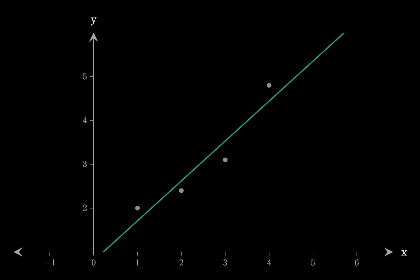
graph#fit-graph{
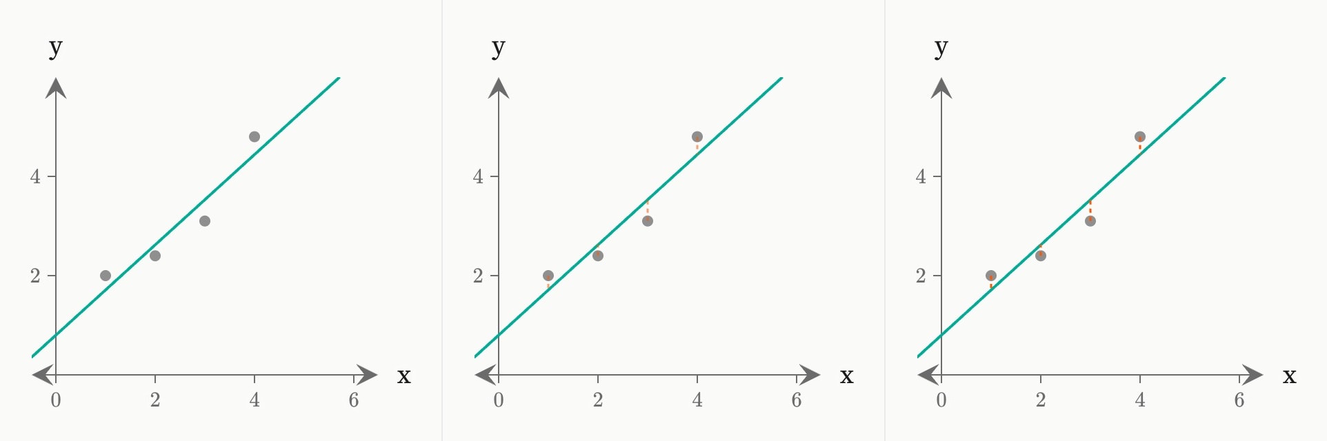
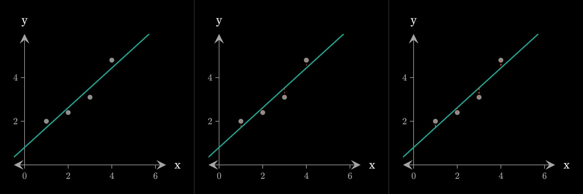
    scatter#observations(x: 1, 2, 3, 4; y: 2.0, 2.4, 3.1, 4.8; colour: grey)
    fit#trend(of: #observations; degree: 1; colour: teal)
    cue{
        residuals(of: #trend; colour: orange)
    }(
        in: 1
    )
}(
    x-axis-label: x
    y-axis-label: y
)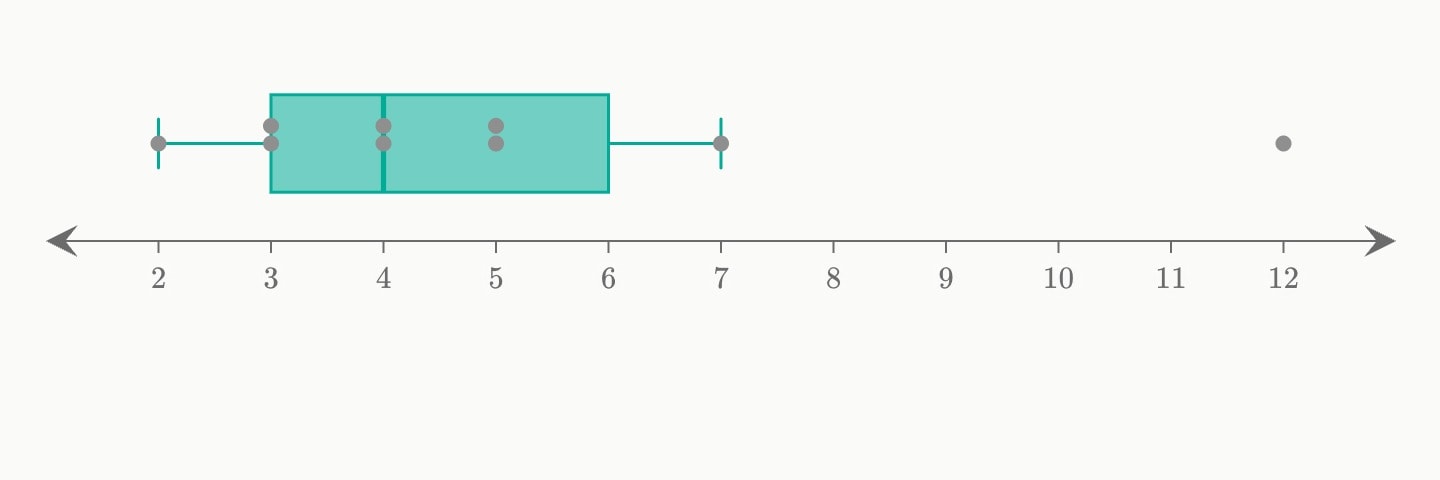
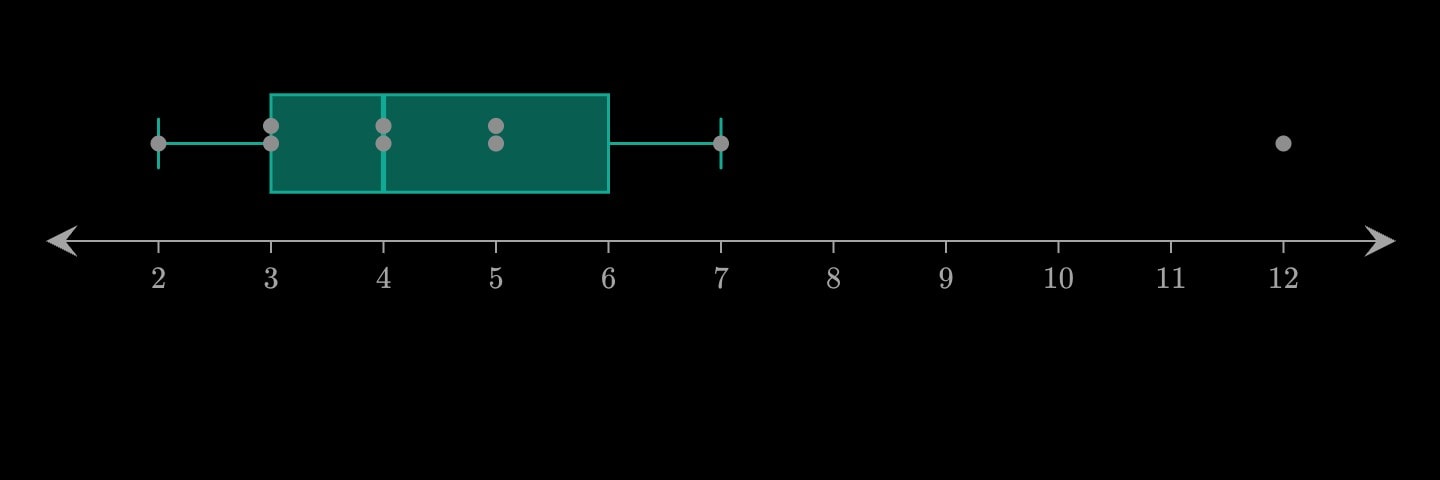
graph:x{
    boxplot(x: 2, 3, 3, 4, 4, 5, 5, 7, 12; colour: teal)
    scatter(x: 2, 3, 3, 4, 4, 5, 5, 7, 12; colour: grey)
}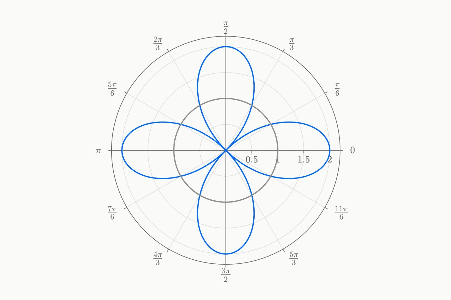
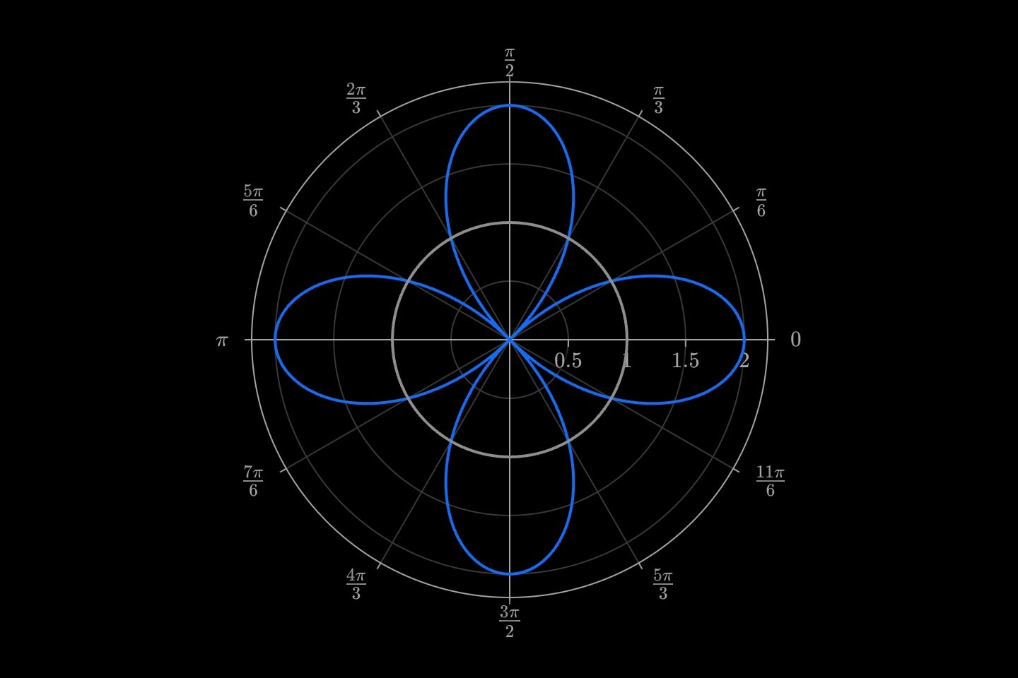
graph:polar{
    curve(expression: 2 * cos(2 * theta); colour: blue)
    curve(expression: 1; colour: grey)
}(
    r-domain: [0, 2.2]
)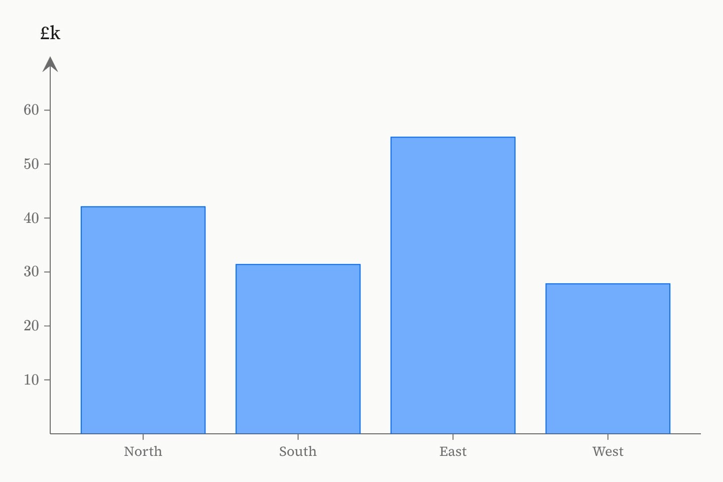
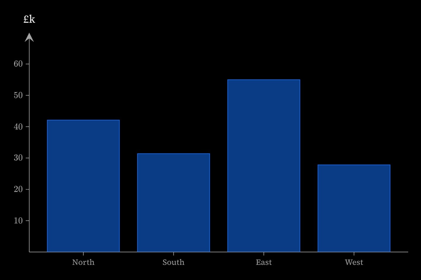
graph{
    bar(x: North, South, East, West; y: 42.1, 31.4, 55.0, 27.8; colour: blue)
}(
    title: Revenue, 2024
    y-axis-label: £k
)#Notes
- An environment's own id is written on the node —
graph#projectile{…}— andcontinue:points at it with#projectile.