Datasets
Declaring a dataset with @data, and reaching it whole, by column, row by row, over time, joined to regions and from packs.
#Declaring a dataset
declares a table of values under an id. Inline, the body is rows of cells separated by |, the first row naming the columns:
@data#islands{
    island     | area   | species
    Baltra     | 25.09  | 58
    Bartolomé  | 1.24   | 31
    Santa Cruz | 903.82 | 444
}
Attached, the implicit value names a .csv file whose header row names the columns: #survey:plants.csv. Nothing downstream can tell the two apart. The id is required — @data: requires an id — datasets are reached as `#id.column` — and a dataset is visible to the whole document, wherever it is written.
#Column names and cells
- Column names are read in lower case, with spaces as hyphens: a header
Species Countis the columnspecies-count. - Every row has as many cells as the header — @data: row 1 has 3 cells; the header declares 2 — and a column name appears once — duplicate column name `a`.
- An inline cell cannot contain
|; there is no escape for it. - A cell is text until the attribute that reads it parses it. A blank cell is kept in its place as an empty cell.
#What a column reads as
A column's kind is decided for the whole column, ignoring blank cells, so a year of daily readings lands on a year of positions rather than on one:
- numeric — every cell a number;
- date — every cell an ISO date,
2024-03-15or2024-03, read as a fractional year: the first of January is the whole year, a month isyear + (month − 1) / 12; - complex — every cell a complex literal such as
4+2i, plain numbers allowed among them; - text — anything else.
Each consumer reads the kind its own way. A graph axis places numbers and dates as positions and text as named categories (graph); a choropleth's values: shades numbers, and a column of words draws nothing.
#The whole dataset
#islands is the whole dataset, accepted where an attribute takes a dataset: table's data: and 's n; a geo dataset in in:.
table(data: #islands; columns: island, area)columns: is a list of plain names, resolved against the table's own data:, so they are written without #. Omitted, every column shows in order. {{#islands}} is refused — an expression needs a column: `{{#d.column}}`.
#One column
#islands.area is one column.
area is the word.A column is a series: one value per row, in row order — the same thing a graph mark's x: or y: takes written out. An attribute of type series accepts either, so scatter(x: 1, 2, 3) and scatter(x: #trial.dose) are the same kind of value, and a column of complex numbers is a complex-series.
#A column as a series
Written bare in an attribute that takes a series, the column is bound — the renderer reads its cells, so the mark follows the data:
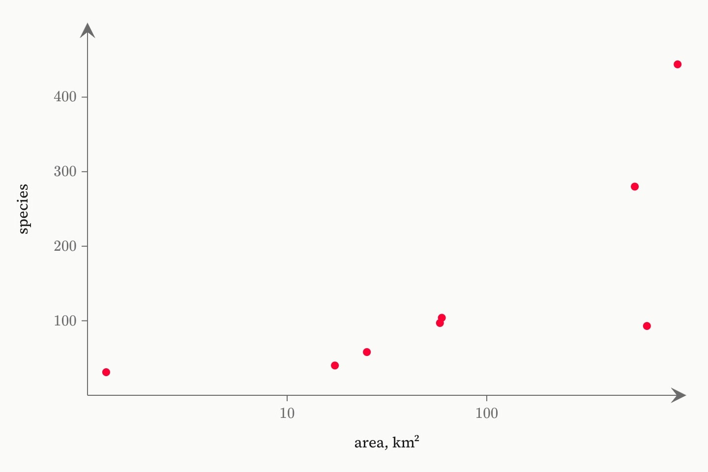
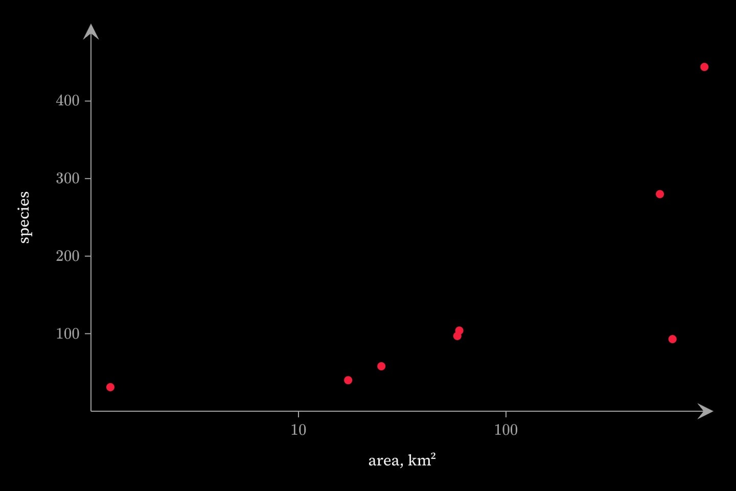
@data#islands{
    island        | area   | species
    Baltra        | 25.09  | 58
    Bartolomé     | 1.24   | 31
    Española      | 58.27  | 97
    Fernandina    | 634.49 | 93
    Genovesa      | 17.35  | 40
    Pinta         | 59.56  | 104
    San Cristóbal | 551.62 | 280
    Santa Cruz    | 903.82 | 444
}

graph{
    scatter(x: #islands.area; y: #islands.species)
}(
    x scale: log
    x axis label: area, km²
    y axis label: species
)- graph marks:
x:,y:and the other series ofscatter,line,bar,polygon,lollipop,histogram,boxplot,violin,density,heatmap, and theirslice:; choropleth'sregions:,values:,colours:,labels:andslice:;marker'slat:,lon:andsize-by:;- a network's
edges(from:,to:,weights:,widths:,groups:,slice:) andvertices(names:,labels:,sizes:,groups:); - the controls'
over:—slider,selectorand their cue twins.
Each attribute takes one column; two columns that belong together, such as x and y, are bound one each.
#A column spliced into text
In a {{…}} expression, a column is its cells as written, joined with a comma and a space, unquoted — in prose, in an attribute, in a line of code:
code{
    lines{
        area = np.array([{{#islands.area}}])
    }
}(
    language: python
)
The splice happens as the document compiles, so an attached file's cells are spliced only where the compiler has the file. Without it, prose shows nothing and a line of code refuses the splice — … which cannot be written into a literal body. A column is a list, so arithmetic on it is refused: a list cannot be used in arithmetic.
#Rows
#Row by row with @for
:#islands repeats its body once per row, top to bottom. {{i}} is the row number from 1 and {{i.<column>}} is that row's cell, spliced as text and parsed by whatever position it lands in:
@data#islands{
    island     | area   | species
    Baltra     | 25.09  | 58
    Bartolomé  | 1.24   | 31
    Santa Cruz | 903.82 | 444
}

@for:#islands{
    {{i}}. {{i.island}} covers {{i.area}} km$^2$ and carries {{i.species}} species.
}
as: renames the binding: (n: #islands; as: row) gives {{row}} and {{row.area}}. A cell is an operand as well as text, so {{row.area * 2}} is arithmetic.
{{row.log-area}} but cannot take part in arithmetic, where the hyphen is a minus.There is no index into a column, so one row is chosen with an in the body:
@for(n: #islands; as: row){
    @if(row.island: Santa Cruz){
        {{row.island}} has {{row.species}} species.
    }
}
The dataset must be declared above the loop — `@for` reads its dataset in document order, so the `@data` must come first. A column is refused as n, with the fix: `#islands.area` names a column, and `@for` goes through rows — loop over `#islands` and write `{{i.area}}` in the body.
#Rows over time
Data with one state per year, month or country is written long: one row per thing per slice, with a column naming the slice. A mark names that column as its slice:, and a control runs over: the same column; the mark draws the rows at the control's value.
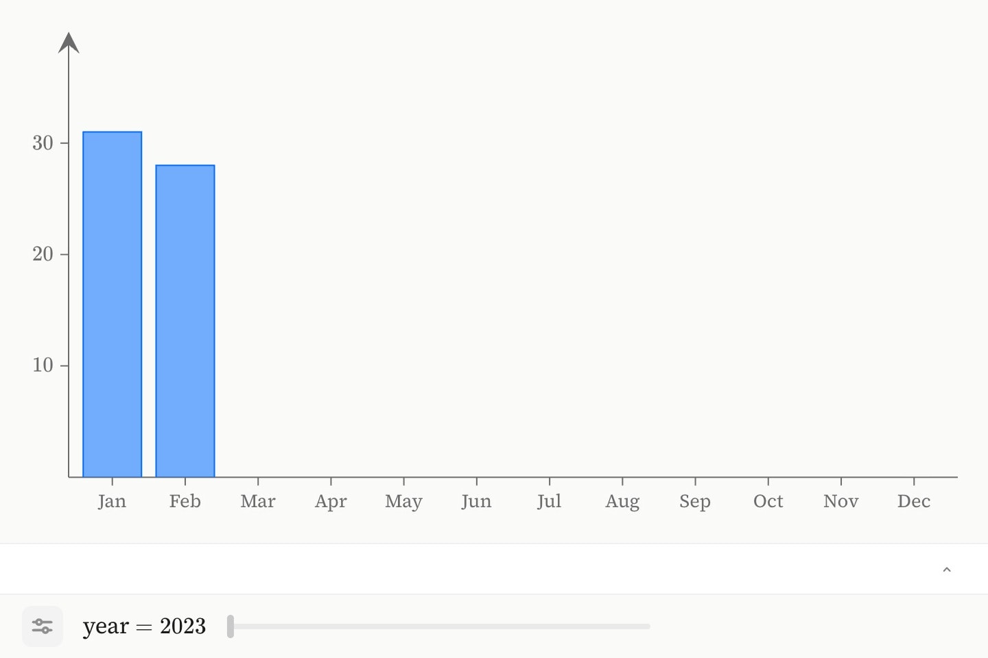
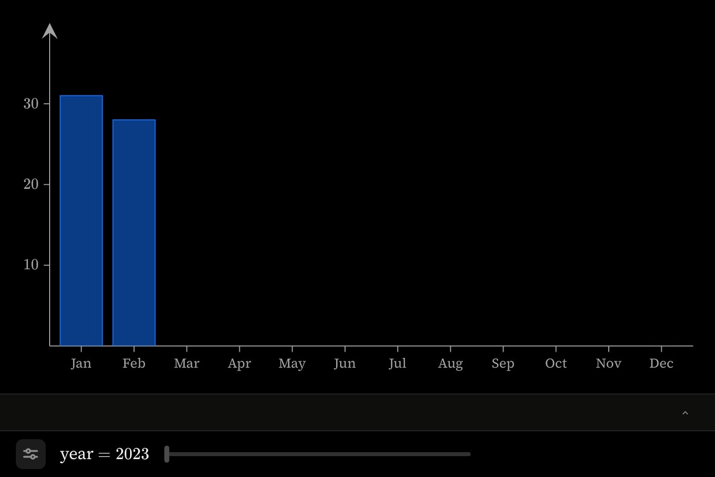
@data#rain{
    year | month | mm
    2022 | Jan   | 80
    2022 | Feb   | 62
    2022 | Mar   | 71
    2023 | Jan   | 95
    2023 | Feb   | 41
    2023 | Mar   | 88
    2024 | Jan   | 58
    2024 | Feb   | 77
    2024 | Mar   | 103
}

graph{
    bar(x: #rain.month; y: #rain.mm; slice: #rain.year)
    slider#year:t(over: #rain.year; discrete)
}(
    y domain: [0, 110]
)
Controls covers how the control takes its stops from the column, and what a mark draws between two of them.
#Maps
#Joining rows to regions
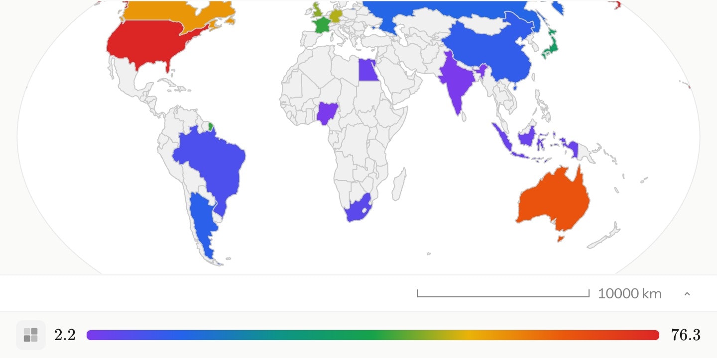
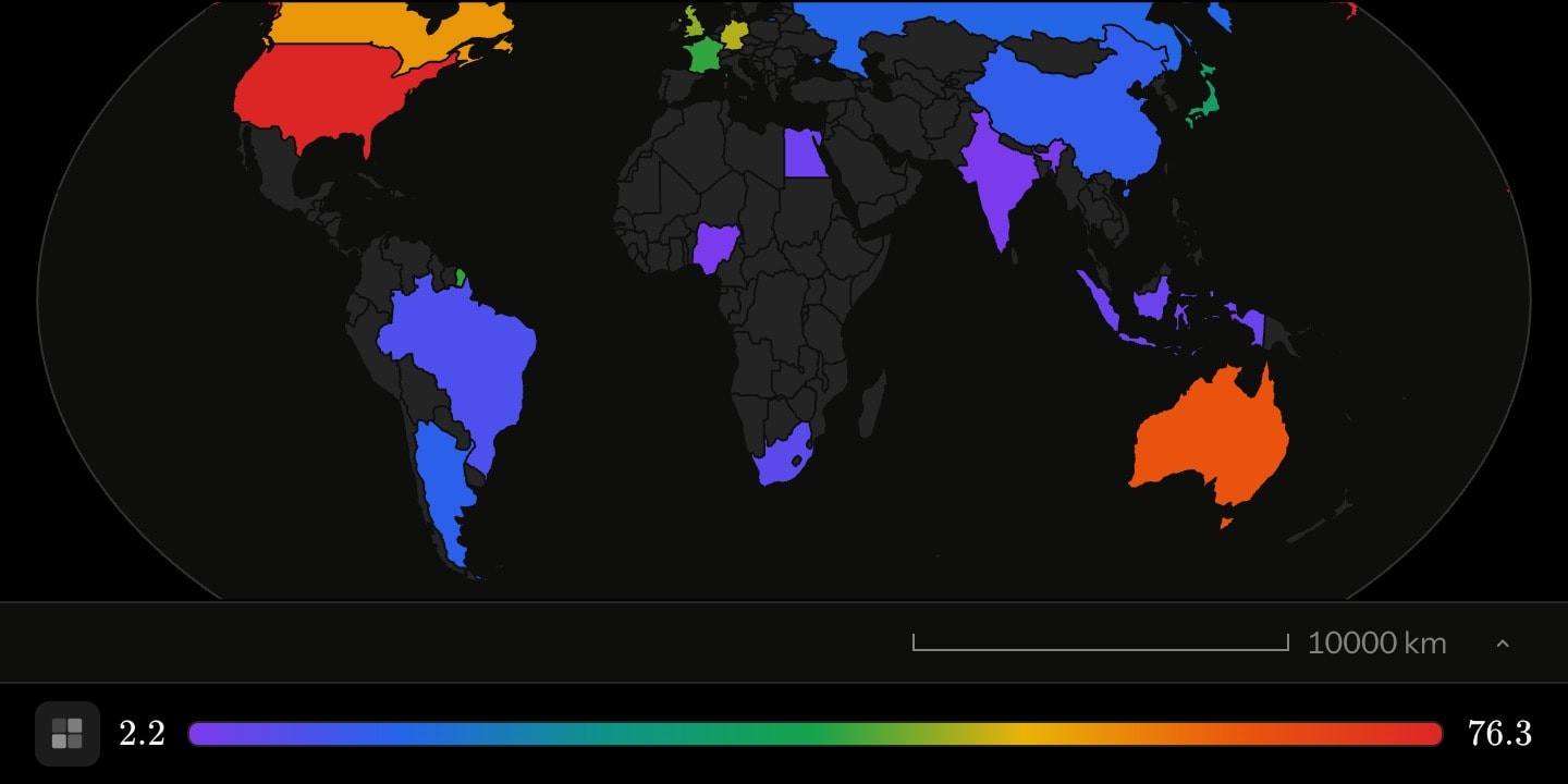
A choropleth joins rows to the regions of its region environment's boundaries: regions: is the column naming each row's region, values: the numbers it is shaded by.
@data#gdp{
    country | gdppc
    France  | 44000
    Germany | 52000
    Spain   | 33000
}

region{
    choropleth(regions: #gdp.country; values: #gdp.gdppc)
}(
    in: world
)
region:world{
    choropleth#gdp(in: world; regions: #economy.country; values: #economy.gdppc)
}#Boundaries as a dataset
An attached .geojson is a geo dataset: boundaries, for regions that are not one of the built-in basemaps. The extension decides the shape — .csv is a table, .geojson boundaries — and a geo dataset is bound whole, as an in::
@data#wards:sydney-wards.geojson
@data#turnout:turnout.csv

region{
    choropleth(in: #wards; regions: #turnout.ward; values: #turnout.pct)
}(
    projection: conic
)
It has no columns and no rows: #wards.name is `#wards` is geo data and has no columns — bind the dataset itself (`attr: #wards`), and :#wards is `#wards` is geo data and has no rows to go through. The feature property that names each region is given on the environment, with names:. Boundaries are only ever attached; an inline body is always a table.
#Datasets from packs
A pack brings datasets in too. makes them reachable through the pack's name, in every way above:
@use:biology

graph{
    line(x: #biology.lynx-hare.year; y: #biology.lynx-hare.hare)
}

@for:#biology.lynx-hare{
    {{i.year}}: {{i.hare}} thousand hares.
}#Provenance and limits
#Where the rows come from
Every row a document shows is in its source: written inline, in an attached file, or in a pack it imports. A reader cannot supply or change rows. Forking an internote copies its source and its attached files, so a fork with other data replaces the declaration or the file it names.
#What a dataset refuses
A dataset holds values as written. There are no computed columns, filters, sorts or aggregates: {{sum(#islands.area)}} is undefined constant `sum`, and {{#islands.area[1]}} is unexpected `[`. A derived column belongs in the file, computed before it is attached, and a filter is an inside a . The declaration itself refuses:
- an attached file that is not
.csvor.geojson— `x.json` has extension `json`, but only csv, geojson are permitted; - a URL — `https://x.org/a.csv` is a URL, but a file path is required;
- both an attached file and an inline body — declare either an inline {grid} body or `src:`, not both.
#Writing guidance
- Checking a document's claims — Every other number worked out, every output quoted from a run, every dataset read and attached whole, every external fact checked and cited, or cut.