@data

#Declaring a dataset

@data declares a named dataset — written once and reached from anywhere in the document. It has one of two shapes, and the shape decides what can be done with it. Tabular is columns of strings. Inline, the body is pipe-delimited rows under a header row that names the columns:

@data#islands{
    island     | area   | species
    Baltra     | 25.09  | 58
    Bartolomé  | 1.24   | 31
    Santa Cruz | 903.82 | 444
}

Attached, a .csv supplies both — @data#survey:galapagos-plants-1973.csv — with src as the implicit attribute and column names taken from the file's header row. Nothing downstream distinguishes the two forms. An id is required in either, because a dataset is reached as #id.column.

#Boundaries as a dataset

The second shape is geo: boundary geometry, attached as a .geojson. It is what a canvas.geo environment draws when the boundaries it needs — electorates, catchments, council wards — are not one of the committed packs. The extension is the format declaration: a .csv is tabular, a .geojson is geo, and .json is not admitted, so the compiler never guesses at a file's shape or reads it to find out.

@data#wards:sydney-wards.geojson
@data#turnout:turnout.csv

canvas.geo{
    choropleth(in: #wards; regions: #turnout.ward; values: #turnout.pct)
}(
    projection: conic
)

A geo dataset is opaque. It has no columns, so it is bound whole — in: #wards — and #wards.name is a compile error that names the fix rather than a lookup that quietly finds nothing. Which feature property names each region is said on the environment consuming it, with names:, because that is a question about the join and not about the file. Only a tabular dataset can be written inline: a { } body is always columns.

#Reaching columns

A tabular dataset's columns are reached by ordinary member access, fully qualified. There is no bare-column shorthand: attribute values are unquoted, so label: island must remain the literal string island. Two mechanisms consume a column, distinguished by the braces:

• {{#survey.area}} — an expression: the cells, joined with commas, resolved while the document compiles. Works in prose, code bodies and attribute values alike.
• #islands / #islands.column — a binding: a reference carried through to the renderer, for attributes typed to accept one.

#Substitution against binding

A column reading resolves at compile time because a dataset is immutable by construction — nothing replaces it and no cell depends on a varying value, so there is nothing for the expression to wait on. A value that does vary at render time — a derived attribute, an animated attribute, a reader-set parameter — makes the expression bound instead of refusing it: {{#fit.slope}} compiles, and ships as a tree the renderer evaluates every frame rather than as compile-time text.

#Tables from data

A table binds a dataset directly and projects columns out of it:

table(data: #islands; columns: island, area, species)

columns: is a list of plain strings the table resolves against its own data: — library-interpreted names rather than references, which is why they are written bare. Every other consumer receives a column as text through substitution: a code environment splices {{#survey.area}} into a numpy array literal.

#Columns as values

Beyond the table, a column is bound where an attribute is typed to take one, and every such attribute takes one column. The consumers:

• The graph's data marks — scatter, line, polygon, bar — take a series per axis, x: and y:, and a slice:.
• choropleth takes regions:, values:, colours:, labels: and slice:; marker takes lat:, lon: and size-by:.
• The controls — slider, selector and their cue twins — take the over: column they run across, anywhere in a scene.
• Everything else — prose, a code environment, an attribute typed for a list — receives a column as text by substitution, {{#survey.area}}.

#One column per attribute

A column binds one attribute, never a pair: scatter(x: #islands.area; y: #islands.species), marker(lat: #cities.lat; lon: #cities.lon). Parallel columns stay row-aligned — a blank cell is kept in place as no value rather than dropped — and where a consumer pairs two columns it drops the pair whose either half it cannot read, so a gap in one column never shifts the readings of the other. The graph marks alone also take a series written out beside a column:

scatter(x: 1, 2, 3; y: 2.0, 2.4, 3.1)
scatter(x: #islands.area; y: #islands.species)
bar(x: North, South, East; y: 42, 31, 55)
choropleth(regions: #gdp.country; values: #gdp.gdppc)

#The two readings of a series entry

A written series entry is read two ways, because the axis it lands on is what decides. A number is a number. 2 * k is an expression of the parameter k — and so, to the expression parser, is Red, which reads as R·e·d. So an entry keeps both its expression and the text it was written as, and the axis picks: on a numeric axis the expression is evaluated, on a categorical one the text is looked up among the axis's names. An entry that is neither — Strongly agree, which no expression grammar accepts — is a name and nothing else.

Which way an undeclared (auto) axis goes follows from that. An entry counts as a name when it is not a number and not an expression whose every letter is a declared parameter; a series with a name on it rules the axis in names, in the order they first appear. So x: a, b beside slider:a and slider:b is two numbers, and beside nothing is two categories. The whole rule is on the graph guide; the consequence for data is that a column of names needs no declaration to be read as names, and a name the axis does not have — under x format: North, South, a row reading West — is a compile error naming the row.

#What a column reads as

A column's kind is decided for the column, not cell by cell: reading 2024-03-15 one cell at a time gives 2024, and a year of daily readings lands on one position. A column is numeric when every non-blank cell is a number; a date when every one is an ISO date, 2024-03-15 or 2024-03, read as a fractional year so that a domain and a fit's slope still speak plain numbers; and text otherwise — names. Each consumer reads the kind its own way. A graph axis takes numbers and dates as positions and labels a date column in whole years under auto; text rules the axis in names, and a text column on an axis declared linear is an error rather than a column of dropped rows. A choropleth shades a numeric values: column through its ramp and enumerates a text one into categories, each with a flat hue. A marker's lat: and lon: are numeric or nothing. Month and weekday names are text like any other, matched by full name or first three letters against the month and weekday presets, and never turned into numbers on the way in.

#Rows over time

Data with a state per slice — per year, per month, per country — is written long-format: one row per thing per slice, with a column saying which slice a row belongs to. A consumer names that column as its slice: — a graph mark, a choropleth — and a control anywhere in the scene names it as its over:. They meet at the column, not at each other. The consumer then shows the slice the parameter holds.

A column with a NUMBER LINE glides: a reader stopped between 2023 and 2024 sees half way, and a thing whose own rows start late or end early holds its nearest reading rather than vanishing. Where the quantity is not a continuous function of the slice — a count of days, a result per election — discrete on a slider makes it stand on one row at a time, and the consumer jumps from slice to slice. A column of NAMES only ever selects, because there is nothing between Brazil and China; a selector is the control for it. A graph's frame is built from every slice at once and holds still as the reader moves through them.

Show code

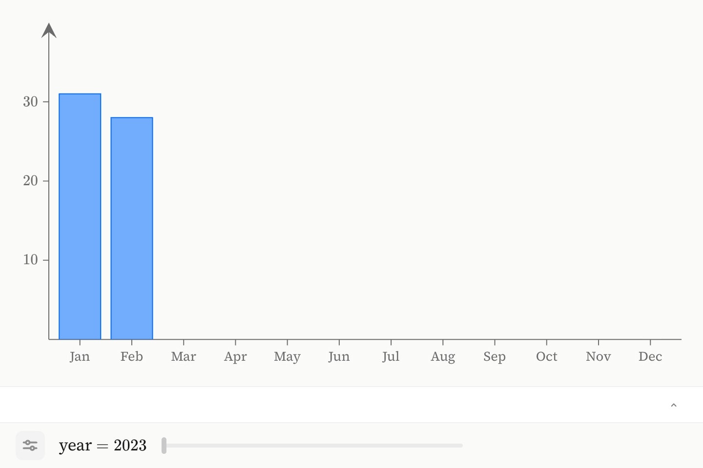
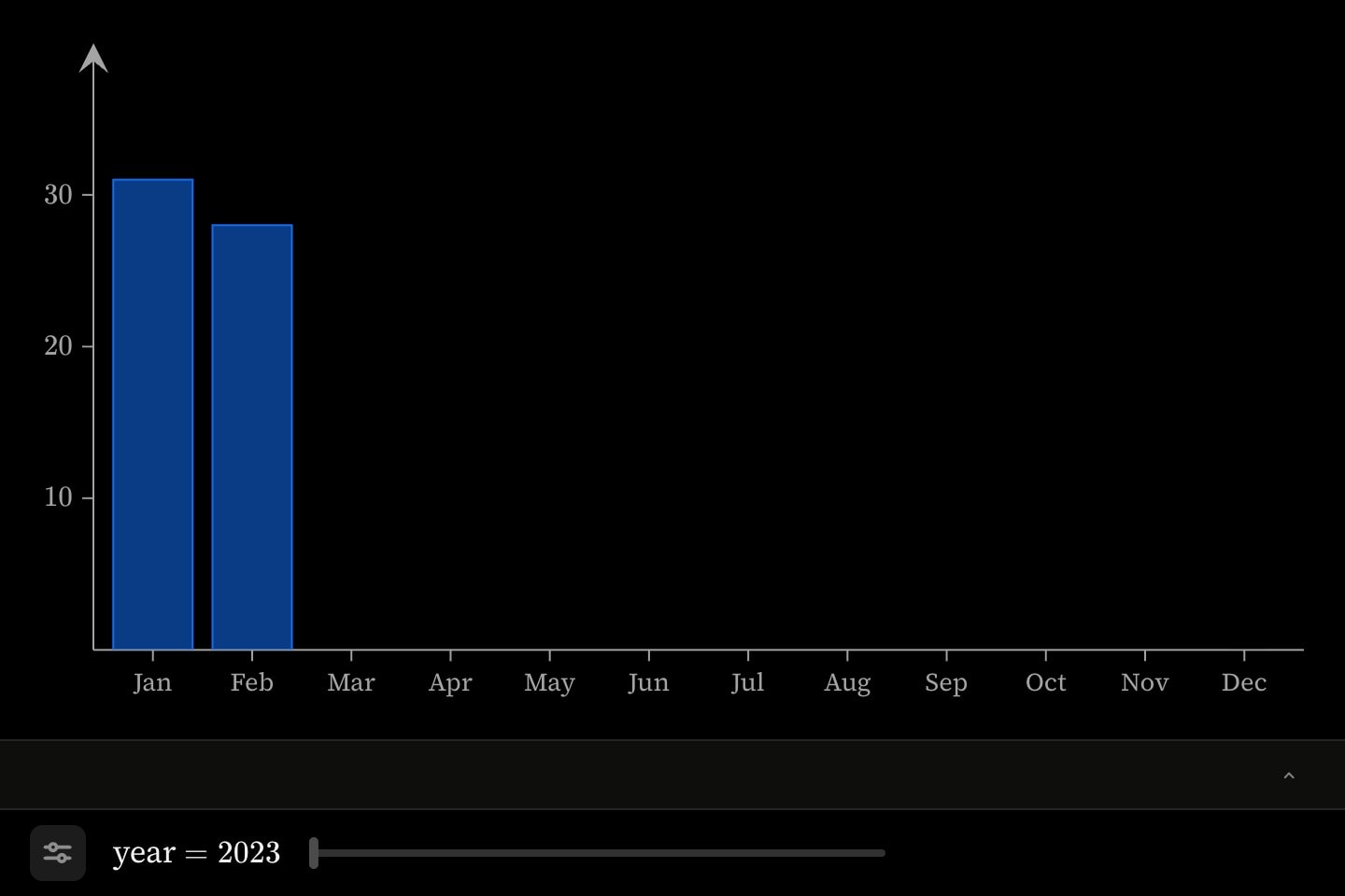
@data#calendar{
    year | month    | days
    2023 | January  | 31
    2023 | February | 28
    2024 | January  | 31
    2024 | February | 29
}

canvas.graph{
    bar(x: #calendar.month; y: #calendar.days; slice: #calendar.year)
    slider#years:t(over: #calendar.year; name: year)
}(
    x format: months
)

The column is read by kind, and the readout reads it back in the same form: years and plain numbers as themselves; ISO dates as fractional years, shown as the nearest day; month and weekday names as their positions, shown by name; HH:MM as hours; YYYY-Www as weeks; text as the words themselves — the same vocabulary a control's format: writes out, which is what to reach for where the cells cannot say (a column of 1…12 that means months). {{#years.value}} cites where the parameter stands in prose. Where a mark's slice: column is not one any parameter names, it reads against the scene's sole bound parameter. Writing a cue control instead hands the moving to the scene.

#One mark per row

Binding a column hands a whole column to one attribute, which is what a scatter or a line wants. The other shape is one mark per row — a parallel-coordinate plot, a box per subject, a card per observation — and that is @for over the dataset itself: @for:#islands walks its rows top to bottom.

@data#islands{
    island     | area   | species
    Baltra     | 25.09  | 58
    Bartolomé  | 1.24   | 31
    Santa Cruz | 903.82 | 444
}

@for:#islands{
    {{i}}. {{i.island}} covers {{i.area}} km$^2$ and carries {{i.species}} species.
}

The loop binding carries both halves of the row. {{i}} is the row number from 1 — the same value @for:3 binds, so it works in prose, in arithmetic ({{i + 1}}) and in an id (#isle-{{i}}) — and {{i.<column>}} is that row's cell, spliced as text and parsed by whatever position it lands in, exactly as if it had been typed there. as: renames both: @for(n: #islands; as: row) gives {{row}} and {{row.area}}. A cell is an operand as well as text, so {{row.area * 2}} is arithmetic on it. A column name with a space follows the usual key spelling — {{i.log area}} or {{i.log-area}}, and the unhyphenated form in arithmetic. A pack's dataset works through its prefix: @for:#statistics.faithful.

canvas.graph{
    @for(n: #soil; as: row){
        line#profile-{{row}}(x: 1, 2, 3; y: {{row.sand}}, {{row.silt}}, {{row.clay}})
    }
}

Rows are the only thing a loop goes through: to work down one column, loop over the dataset and read that column. There is no filter and no sort — an @if inside the body is the filter. The dataset has to be declared above the loop, since n is read as the document compiles; naming a column there (@for(n: #islands.area)) is refused and points at {{i.area}}; so are a geo dataset, which has no rows, and an attached file this build cannot read — refused rather than run zero times, which would let one document mean two things. Cells are substituted at compile time, and a dataset cannot change, so nothing a loop writes can go stale.

#Scope and limits

• Directives have no placement rules — a @data is document-visible wherever it is written, including inside an @included partial. A @for over one is the exception: it reads the rows as it compiles, so the @data must come first.
• Attached data is .csv or .geojson, and nothing else — not .json, not a URL.
• No inline geo data. Boundaries arrive as a file.
• No computed columns, row filters or aggregates on a tabular dataset. A transform belongs upstream, stored in the data, which keeps column access a pure lookup and columns substitutable; the one thing that iterates is @for, and its filter is an @if in the body.
• @data holds tables of values; @let holds scalars and repeated fragments.