network
A canvas environment that draws a network of vertices and edges, such as a social or citation network.
networkOn this page
#Vertices, edges and direction
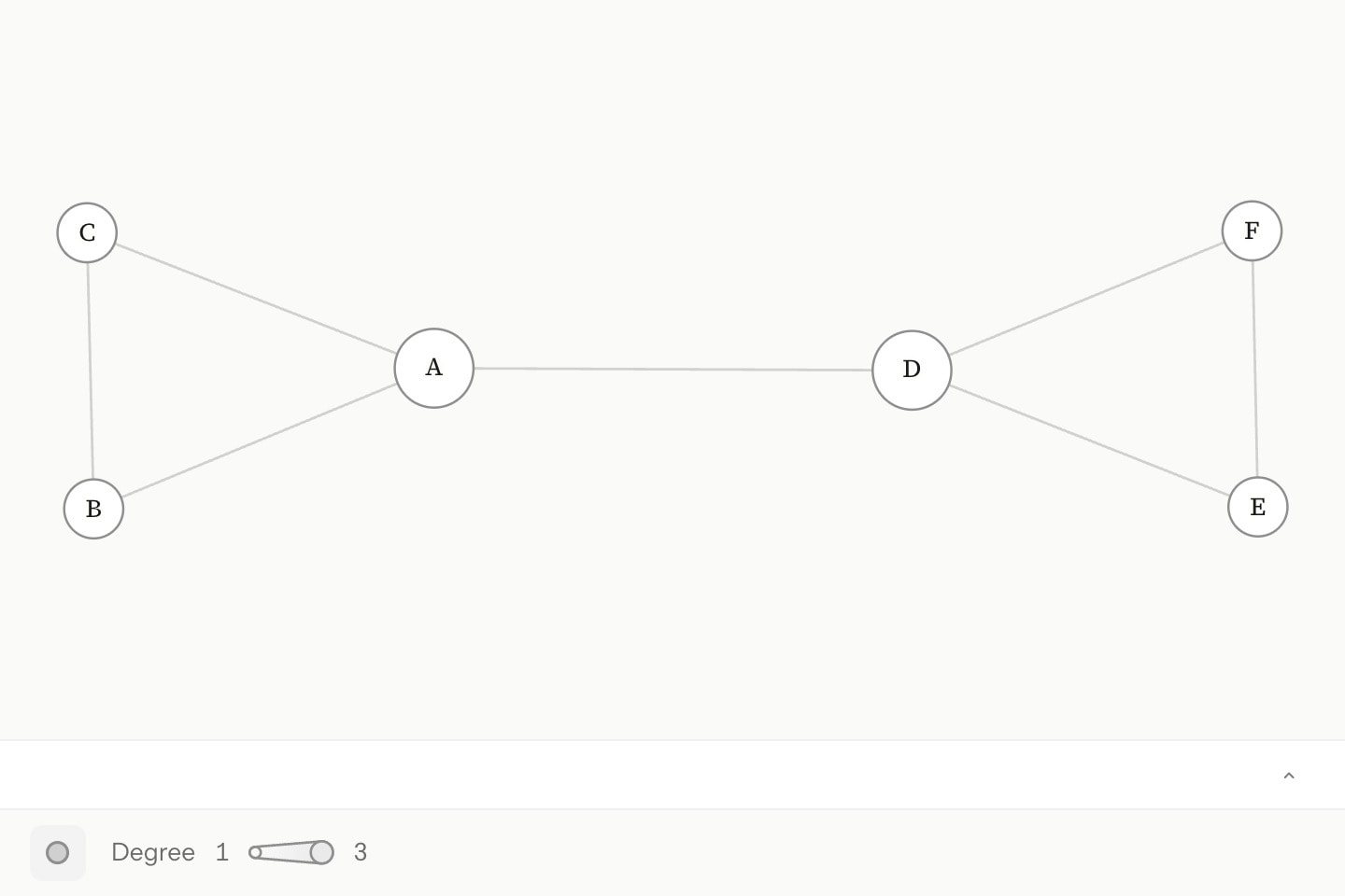
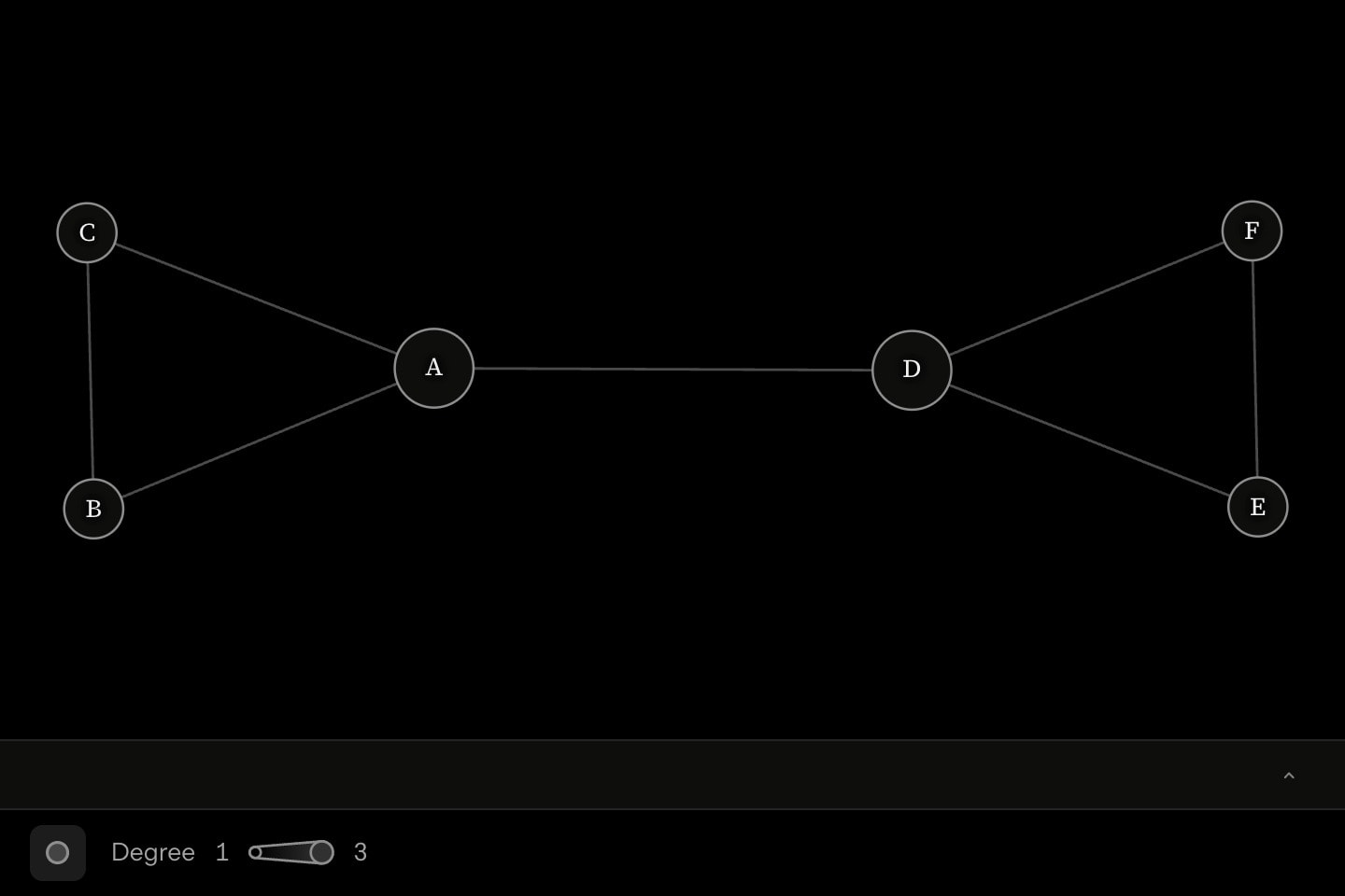
network draws a graph in the discrete-maths sense: a social or citation network, a food web, a causal loop. A vertex is a point whose body is its label, and an edge joins two vertices by their ids. The environment places the vertices and measures what was written. A flowchart also joins things with arrows; it routes them round boxes of text and measures nothing.
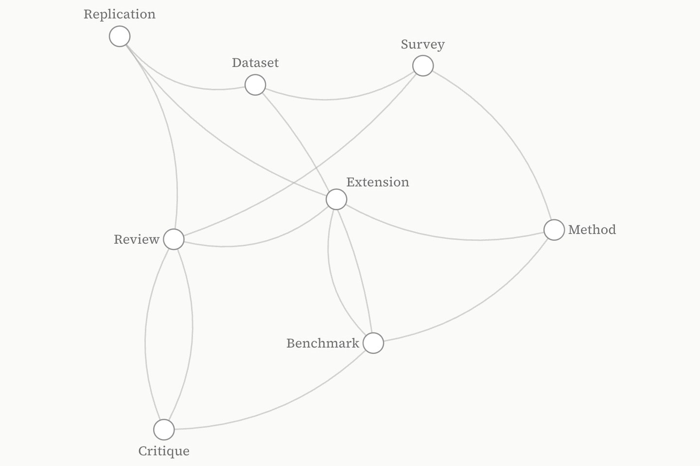
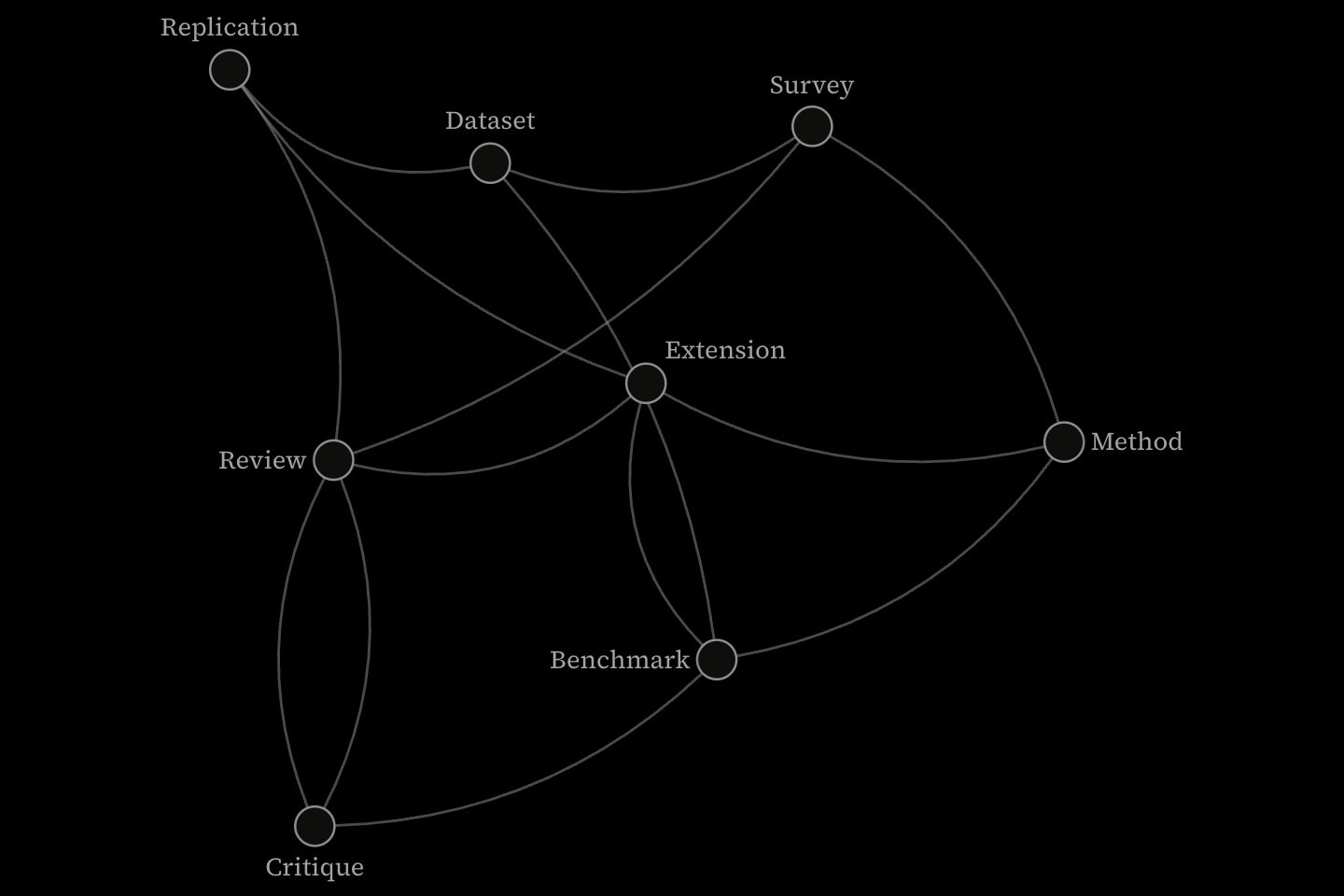
directed is none unless written, and the network is undirected. directed: arrows makes every edge run from from to to: edges carry heads, in- and out-degree are counted apart, and a path follows the edges' direction. directed: curves is the same directed network with no heads, each edge bowing to the right of the way it runs, so two vertices that point at each other are joined by two separate curves; on a crowded network it keeps heads from piling up round every popular vertex.
@data#citations{
    paper       | cites
    Critique    | Review
    Method      | Survey
    Dataset     | Survey
    Benchmark   | Method
    Benchmark   | Dataset
    Extension   | Method
    Extension   | Benchmark
    Critique    | Benchmark
    Replication | Extension
    Replication | Dataset
    Review      | Extension
    Review      | Critique
    Review      | Replication
    Review      | Survey
}

network{
    edges(from: #citations.paper; to: #citations.cites)
}(
    directed: curves
)
Two edges between the same pair bow apart, and an edge from a vertex to itself is a loop over it. sign: positive or negative sets a + or − along an edge near its end, and shape: none draws a vertex as its words alone: together, a causal-loop diagram.
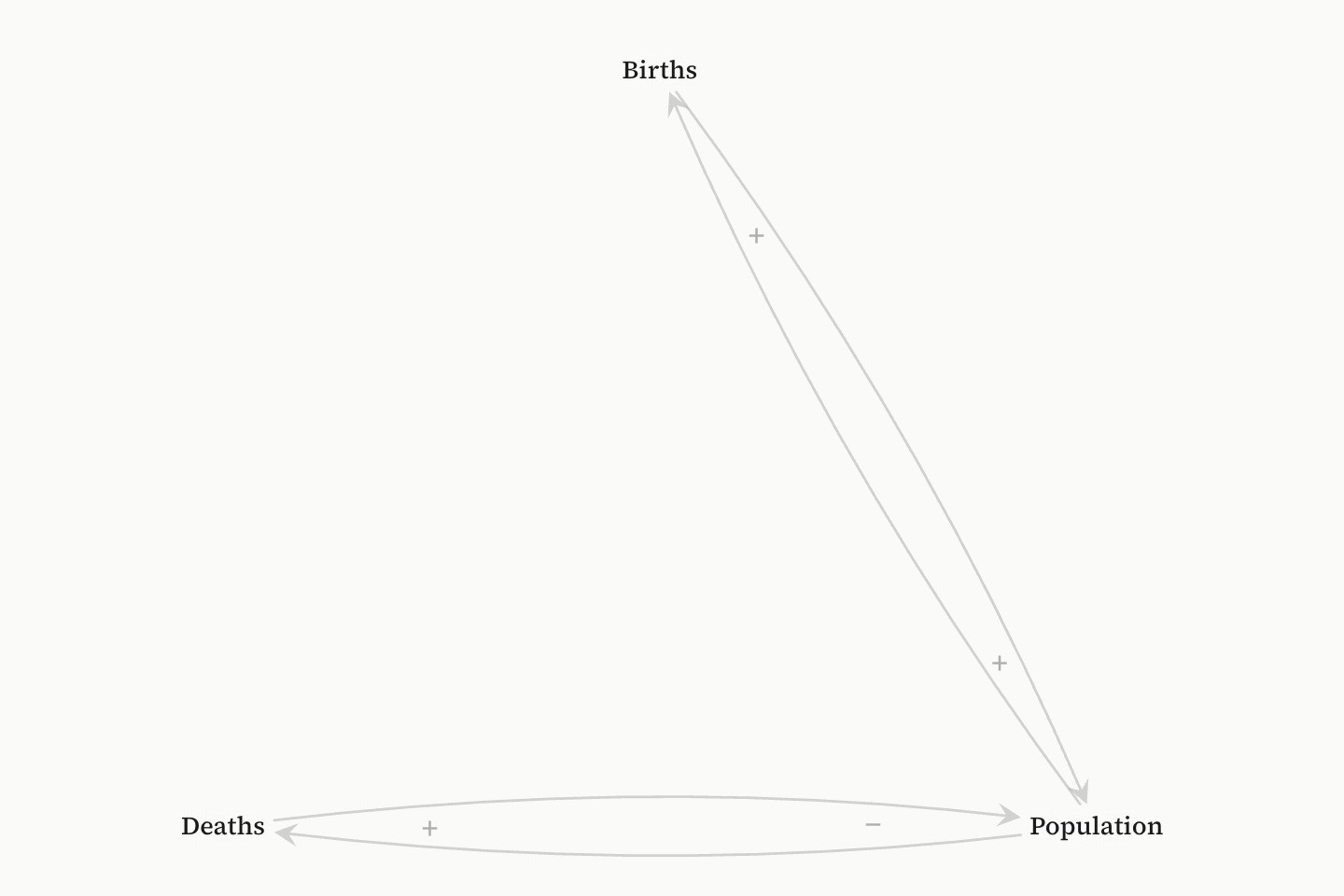
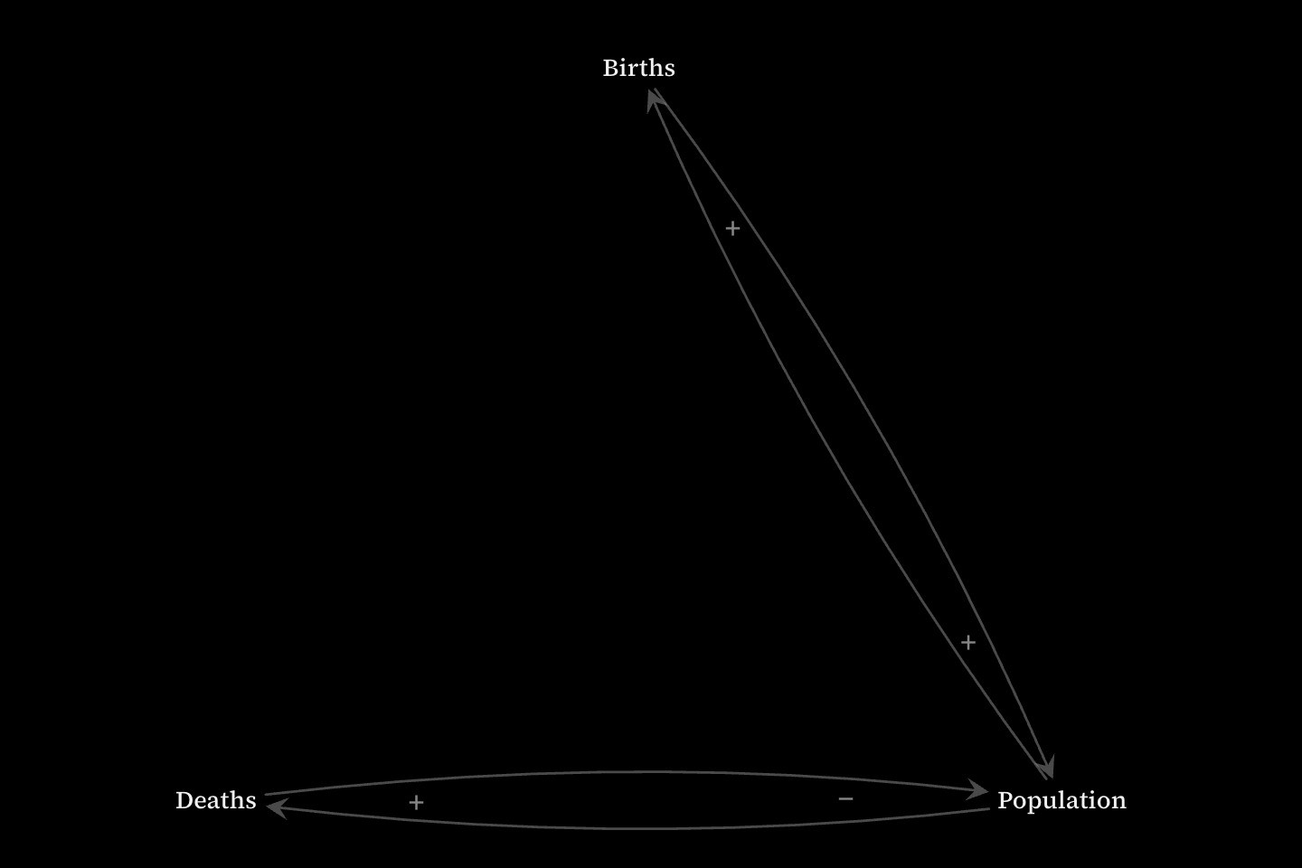
network:circle{
    vertex#births{Births}(shape: none)
    vertex#population{Population}(shape: none)
    vertex#deaths{Deaths}(shape: none)

    edge(from: #births; to: #population; sign: positive)
    edge(from: #population; to: #births; sign: positive)
    edge(from: #population; to: #deaths; sign: positive)
    edge(from: #deaths; to: #population; sign: negative)
}(
    directed: arrows
)
An edge's weight is what the network measures it by: the length a path adds up and the weight a vertex is sized by. A weight cannot be negative; a relation that opposes is sign: negative. show weights labels every weighted edge that has no label of its own with its weight.
#Layouts
layout is the implicit attribute, so network:circle{…} names its layout in the head. There are eight.
force, the default, draws connected vertices together and pushes every vertex away from the others, from starting places drawn fromseed. The same network and seed come out the same every time; a different seed, or adding or reordering vertices, is a different arrangement. Separate pieces are laid out apart and packed largest first.circlesets the vertices clockwise round a ring from the top, eachgroupkept together in the order its first vertex is written.gridsets them in rows in the order written.treehangs a spanning tree fromroot, each parent centred over its children.binary-treehangs a tree whose children are left and right (below).layeredranks a directed network so its edges run one way, an edge that closes a cycle left running back; on an undirected network it ranks the vertices by their distance fromroot.bipartitesets the two sides of a two-sided network on two ranks: the twogroups when every vertex has one and there are exactly two, the first met on the top rank; otherwise the two sides a two-colouring finds.chorddraws each vertex as an arc of a ring and each edge as a ribbon across it (below).
Without root, a tree hangs from the first vertex written, or on a directed network the first nothing points into. The four ranked layouts run down; direction: right turns them on their side.
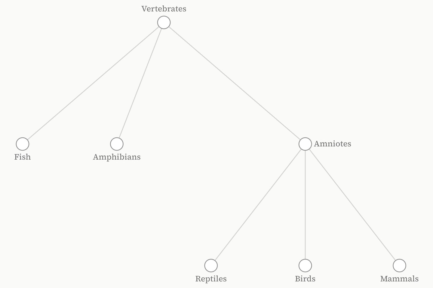
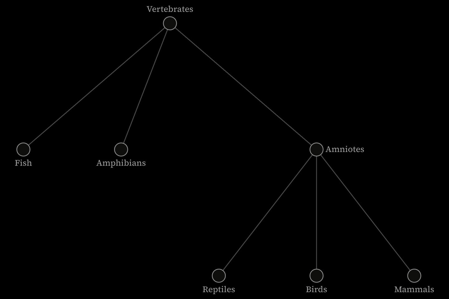
network:tree{
    vertex#vertebrates{Vertebrates}
    vertex#fish{Fish}
    vertex#amphibians{Amphibians}
    vertex#amniotes{Amniotes}
    vertex#reptiles{Reptiles}
    vertex#birds{Birds}
    vertex#mammals{Mammals}

    edge(from: #vertebrates; to: #fish)
    edge(from: #vertebrates; to: #amphibians)
    edge(from: #vertebrates; to: #amniotes)
    edge(from: #amniotes; to: #reptiles)
    edge(from: #amniotes; to: #birds)
    edge(from: #amniotes; to: #mammals)
}(
    root: #vertebrates
)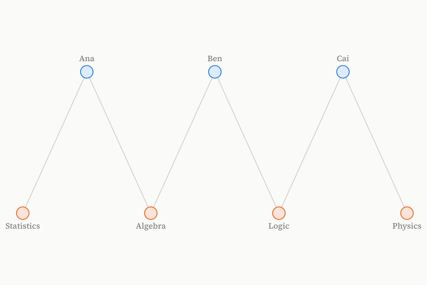
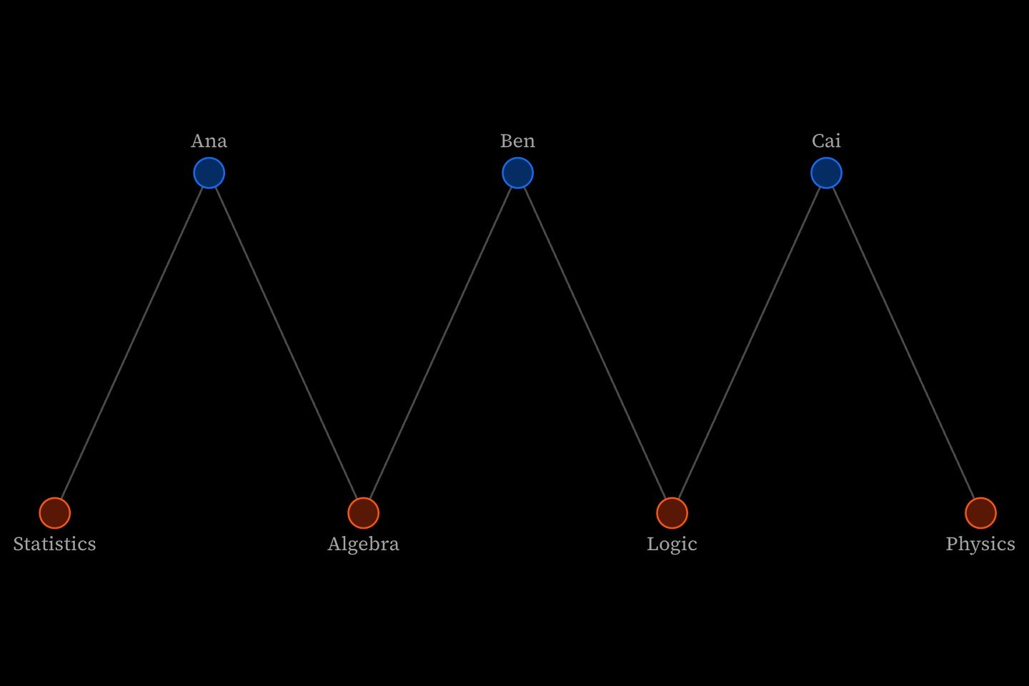
network:bipartite{
    vertex#ana:students{Ana}(colour: blue)
    vertex#ben:students{Ben}(colour: blue)
    vertex#cai:students{Cai}(colour: blue)
    vertex#stats:modules{Statistics}(colour: orange)
    vertex#algebra:modules{Algebra}(colour: orange)
    vertex#logic:modules{Logic}(colour: orange)
    vertex#physics:modules{Physics}(colour: orange)

    edge(from: #ana; to: #stats)
    edge(from: #ana; to: #algebra)
    edge(from: #ben; to: #algebra)
    edge(from: #ben; to: #logic)
    edge(from: #cai; to: #logic)
    edge(from: #cai; to: #physics)
}#Binary trees and branch lengths
binary-tree places a vertex's first child, by the edge written first, to its left and the rest to its right, and gives every vertex a column of its own in that order, so a search tree's keys read off left to right. A lone child stands to the left; a lone right child is written after a hidden vertex that holds the left place.
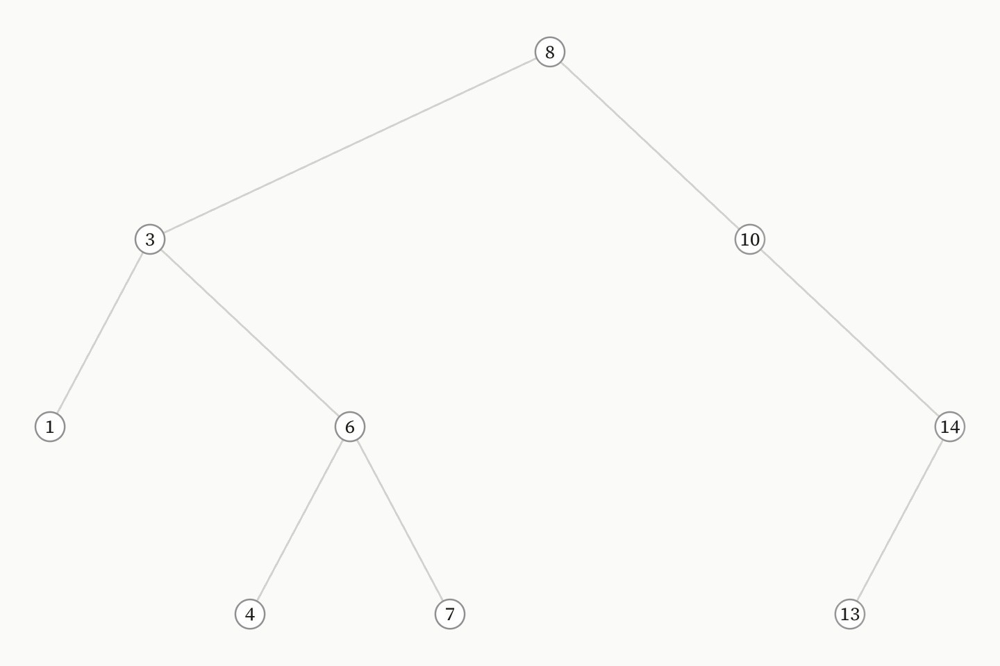
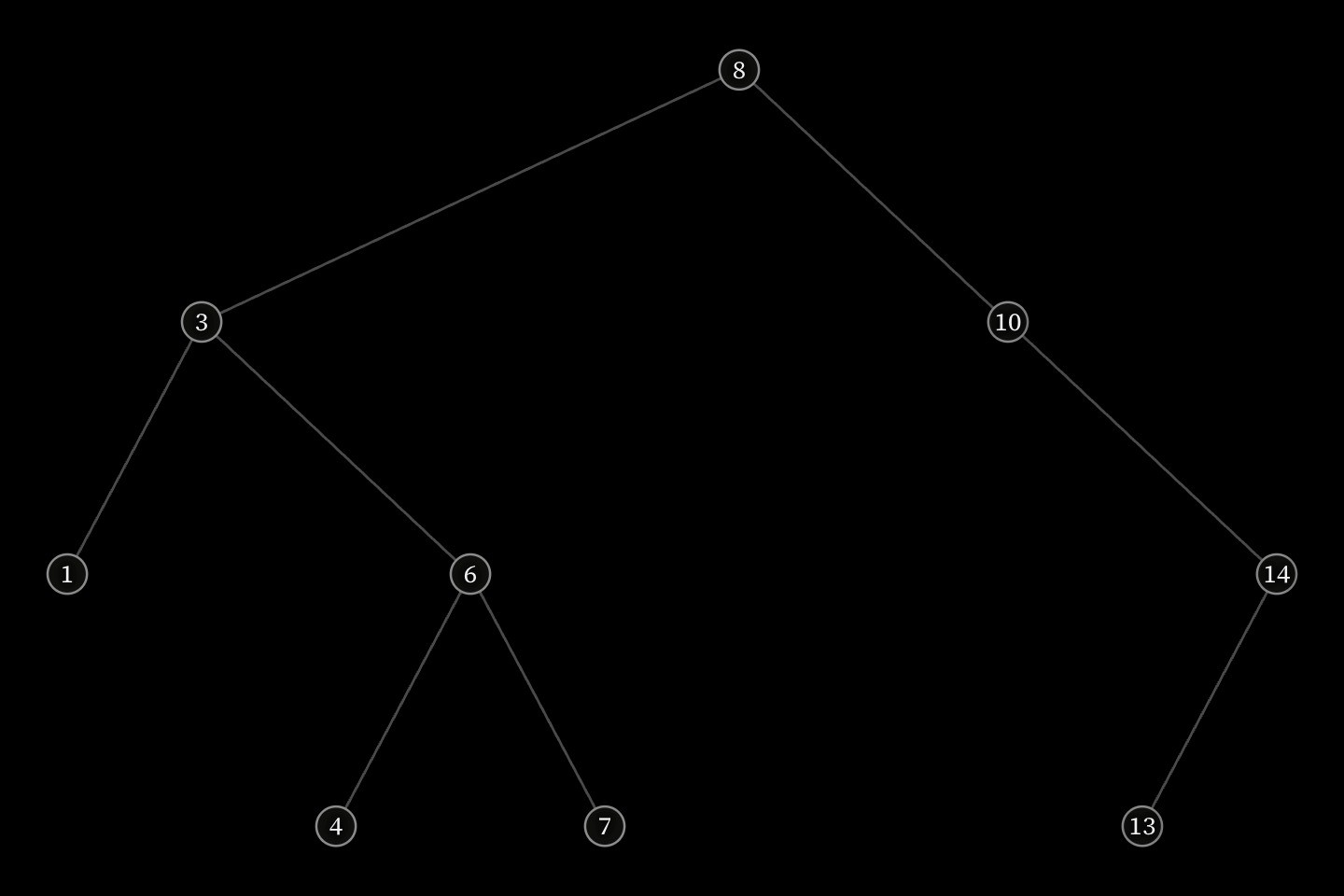
network:binary-tree{
    vertex#k8{8}
    vertex#k3{3}
    vertex#k10{10}
    vertex#k1{1}
    vertex#k6{6}
    vertex#gap(hidden: true)
    vertex#k14{14}
    vertex#k4{4}
    vertex#k7{7}
    vertex#k13{13}

    edge(from: #k8; to: #k3)
    edge(from: #k8; to: #k10)
    edge(from: #k3; to: #k1)
    edge(from: #k3; to: #k6)
    edge(from: #k10; to: #gap)
    edge(from: #k10; to: #k14)
    edge(from: #k6; to: #k4)
    edge(from: #k6; to: #k7)
    edge(from: #k14; to: #k13)
}(
    root: #k8
)
In either tree, edges(length by: weight) makes each edge as long as its weight, an unweighted edge counting 1, so a vertex stands as far from the root as the weights on the way down add up to: a phylogram or a dendrogram, whose leaves line up by themselves. edges(shape: elbow) draws each edge square, across at its parent's rank and then along the flow, so only the run along the flow carries length. The compiler warns when either is written on a layout that cannot use it.
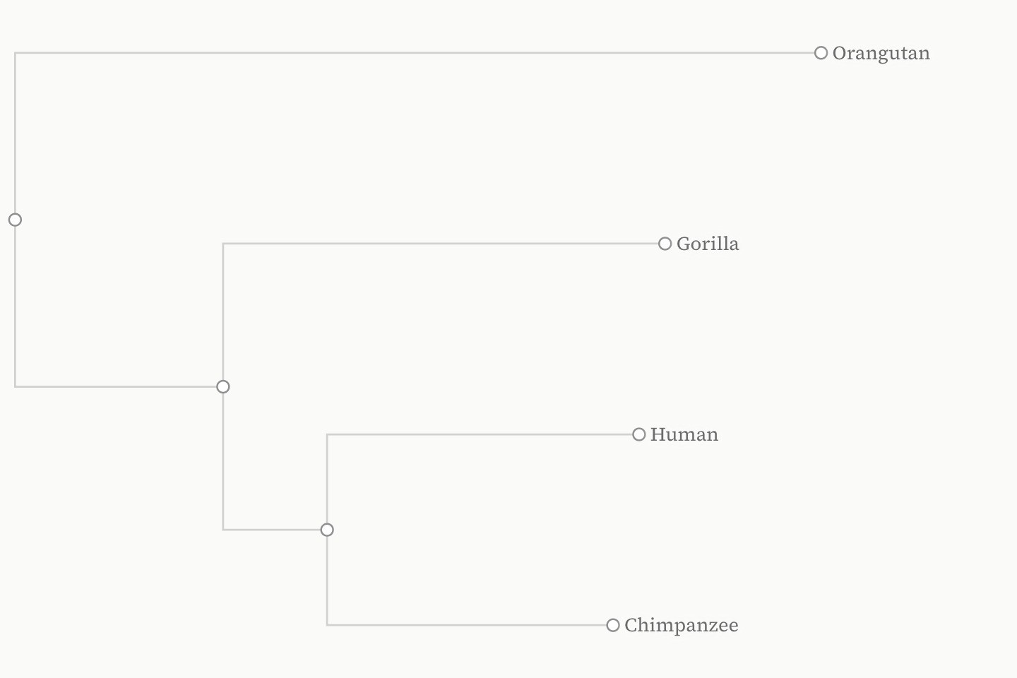
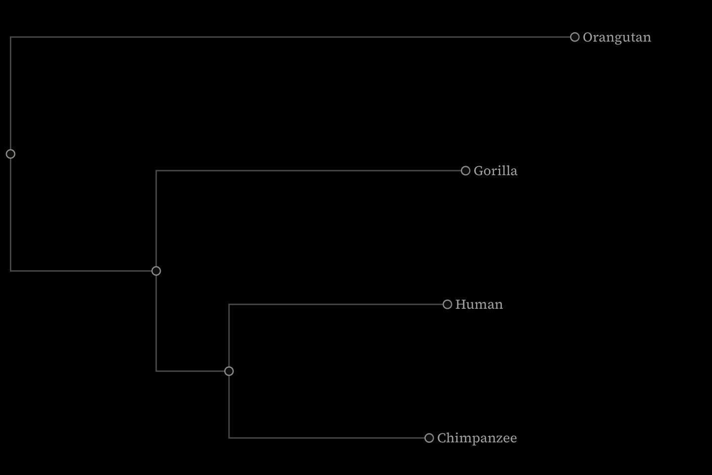
network:tree{
    vertex#human{Human}(size: 0.4)
    vertex#chimp{Chimpanzee}(size: 0.4)
    vertex#gorilla{Gorilla}(size: 0.4)
    vertex#orang{Orangutan}(size: 0.4)
    vertex#root(size: 0.4)
    vertex#hcg(size: 0.4)
    vertex#hc(size: 0.4)

    edge(from: #root; to: #orang; weight: 0.31)
    edge(from: #root; to: #hcg; weight: 0.08)
    edge(from: #hcg; to: #gorilla; weight: 0.17)
    edge(from: #hcg; to: #hc; weight: 0.04)
    edge(from: #hc; to: #human; weight: 0.12)
    edge(from: #hc; to: #chimp; weight: 0.11)

    edges(length-by: weight; shape: elbow)
}(
    root: #root
    direction: right
)#Chord diagrams
chord draws a network of flows, such as migration or trade between regions. Each vertex is an arc of a ring, as long as the flows into and out of it together, and each edge is a ribbon across the ring whose two ends are its weight's share of the arcs it joins; an edge with no weight counts 1. Within an arc the ribbons stand in the order of where they go, so none cross where they leave it, and a flow from a vertex to itself loops back onto its own arc. The vertices go round in the order circle sets them, and their names stand outside the ring.
On a network with directed: arrows, a ribbon leaves the arc it starts from and stops short of the arc it reaches, and takes the colour of the vertex it leaves; an edge list's colour or colour-from overrides that. A sliced edge list resizes the arcs to each slice's flows.
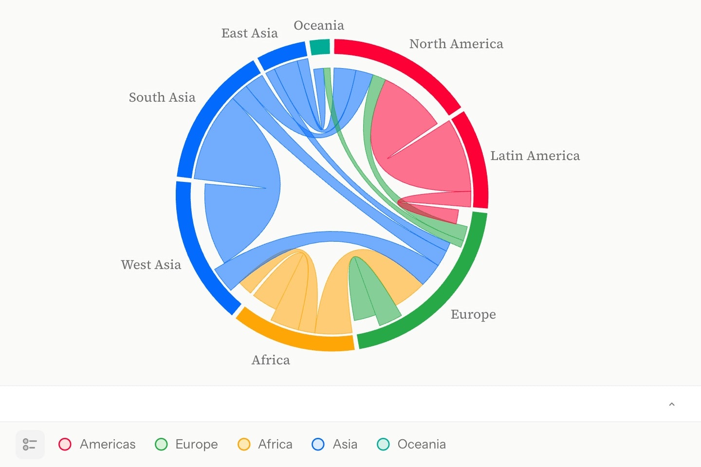
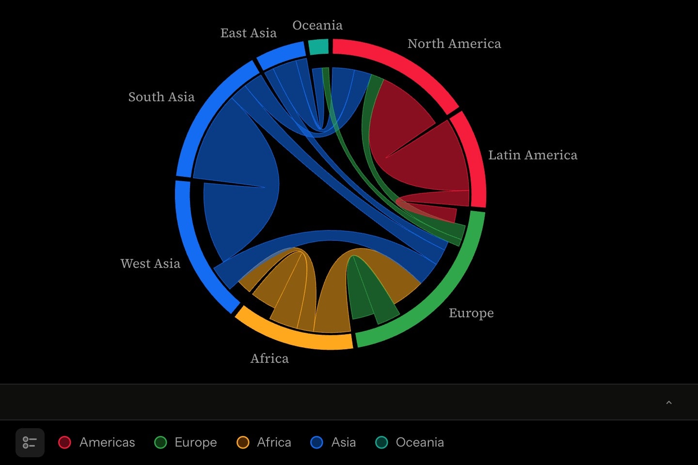
@data#regions{
    name          | continent
    North America | Americas
    Latin America | Americas
    Europe        | Europe
    Africa        | Africa
    West Asia     | Asia
    South Asia    | Asia
    East Asia     | Asia
    Oceania       | Oceania
}

@data#flows{
    origin        | destination   | millions
    Latin America | North America | 6.2
    South Asia    | West Asia     | 7.5
    Africa        | Europe        | 3.1
    South Asia    | North America | 1.6
    East Asia     | North America | 2.0
    Europe        | North America | 1.2
    Africa        | West Asia     | 1.4
    South Asia    | Europe        | 1.5
    East Asia     | Oceania       | 0.9
    Europe        | Oceania       | 0.6
    West Asia     | Europe        | 2.2
    Latin America | Europe        | 1.3
    East Asia     | Europe        | 0.8
    Africa        | Africa        | 2.4
    Europe        | Europe        | 2.0
}

network:chord{
    vertices(
        names: #regions.name
        colour: #regions.continent -> (Americas: red; Europe: green; Africa: yellow; Asia: blue; Oceania: teal)
    )
    edges(from: #flows.origin; to: #flows.destination; weights: #flows.millions)
}(
    directed: arrows
)
A chord sizes and places everything by its flows, so a vertex's size, shape and at, an edge list's width, a path and directed: curves are refused (canvas/network-chord).
#Placing a vertex by hand
A vertex with at sits at that point of the frame, written as two fractions from 0 to 1 from the top-left, y down. The force layout arranges the other vertices around it; the other layouts place the rest as if it were in its own slot, which is left empty. at is animatable, and the layout reads its first value, so a keyframe moves that vertex alone.
#Networks from @data
edges binds an edge list from a dataset: one edge per row, endpoints named by the from and to columns, with weights from a third. Each distinct cell is a vertex labelled with its text, and a row with a blank endpoint is dropped. vertices binds a vertex table: one vertex per row, keyed by names, which the edge list's cells are matched against. A vertex in the table with no edges is drawn on its own.
An inline vertex whose label or id matches a name, case and spacing aside, is that vertex, which is how a data vertex is coloured, pinned, or given an id to cite or to point a path at. Inline edges, edge lists and vertex tables mix freely. Several environments can bind the same dataset; each builds and measures its own network.
#Drawing the data on the network
Colour, size and shape are set on the tables, not on the environment, so each table's rows follow their own rule. A vertex table takes colour, size and shape; an edge list takes colour and width. Each is a style attribute — a look, a list of looks, or a reading applied with -> to a map, a ramp or an expression — as Styling marks from data sets out. A column of categories is applied to a map, colour: #people.team -> (design: teal; research: orange; otherwise: grey); a category the map does not name takes its otherwise, or without one the plain look. Inline vertices are coloured by their own group through colour: #self.group -> (core: teal; otherwise: grey). A numeric column is applied to an interval and a size: size: #cities.population -> 0..3 -> 1 + _ draws 0 at the plain size and 3 at twice it, in multiples of the plain vertex, and a width's sizes are in pixels. A column of numbers alone, width: #roads.lanes, is the sizes as written.
An edge list can instead colour each edge from the vertices it joins, with colour-from: ends in the colour its two ends share, and an even mix where they differ; gradient from the colour of the vertex it leaves to the colour of the one it reaches; from in the colour of the vertex it leaves; none, the default, leaves the edge its own colour.
A vertex's own colour and shape win over what its table gives it.
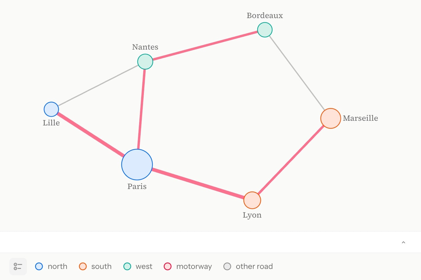
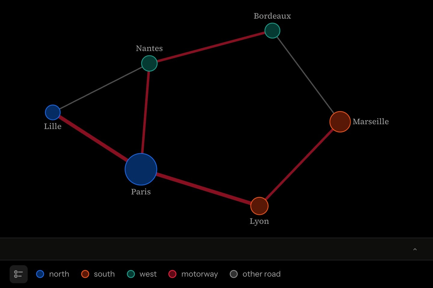
@data#cities{
    city      | population | region
    Paris     | 2.10       | north
    Lille     | 0.24       | north
    Lyon      | 0.52       | south
    Marseille | 0.87       | south
    Bordeaux  | 0.26       | west
    Nantes    | 0.32       | west
}

@data#roads{
    from      | to        | km  | lanes | kind
    Paris     | Lille     | 225 | 6     | motorway
    Paris     | Lyon      | 465 | 6     | motorway
    Lyon      | Marseille | 315 | 4     | motorway
    Paris     | Nantes    | 385 | 4     | motorway
    Nantes    | Bordeaux  | 345 | 4     | motorway
    Bordeaux  | Marseille | 645 | 2     | other road
    Lille     | Nantes    | 590 | 2     | other road
}

network{
    vertices(
        names: #cities.city
        colour: #cities.region -> (north: blue; south: orange; west: teal)
        size: #cities.population -> 0..2.1 -> 1 + 1.5_
    )
    edges(from: #roads.from; to: #roads.to; weights: #roads.km; width: #roads.lanes; colour: #roads.kind -> (motorway: red; other road: grey))
}
weights and width are different claims. A weight is what the network measures an edge by, here the kilometres, and width is only drawn: the lanes, which make a road look major without making it any shorter.
The footer keys each key of a colour map beside its hue, and its shape where a shape map follows the same reading, vertex and edge alike, with a map's otherwise as other. A vertex size or edge width applied to a measurement, #self.degree -> 1..10 -> 1 + 2_, is keyed as a wedge across its interval; a column's sizes are not. An edge coloured from its ends is not keyed. !legend turns the key off.
Labels are set inside the vertices when every labelled vertex can hold its own, and otherwise all beside, each on a side its edges leave clear without covering another vertex, edge or label or leaving the frame. A label with no room shows on hover. Hovering a vertex fades everything outside its reach: on a directed network what lies downstream of it, on an undirected one its whole connected piece.
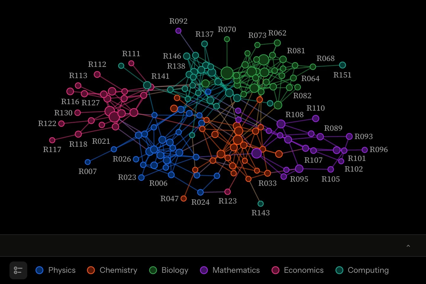
Two bindings draw a network as large as its data. Below, 160 researchers and the 342 co-author pairs among them, generated for the example rather than collected, each vertex sized by its researcher's papers and coloured by department.
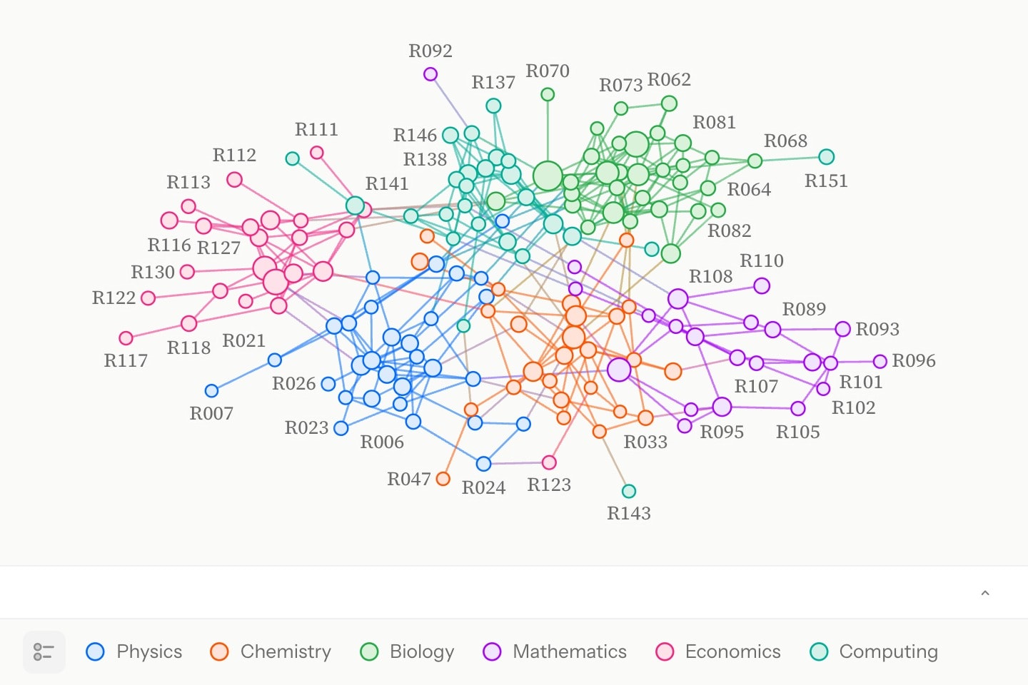
network{
    vertices(
        names: #researchers.name
        colour: #researchers.department -> (Physics: blue; Chemistry: orange; Biology: green; Mathematics: purple; Economics: pink; Computing: teal)
        size: #researchers.papers -> 0..63 -> 1 + 1.5_
    )
    edges(from: #coauthors.a; to: #coauthors.b; colour-from: ends)
}#Slicing an edge list
edges(slice: …) names a column that sorts an edge list's rows into slices, years or named periods, and a slider or selector whose column: is the same column shows one slice at a time. On a slider, the slice shown is the last at or before its value. Rows naming the same pair the same way round are one edge, taking its weight and the row its style attributes read from its first row. As the slice changes, the network settles to that slice's edges, the vertices gliding to their new places, and the edges fade in and out. The measurements count every slice.
network{
    cue.slider#year:t(column: #ties.year; name: Year; at: 1; duration: 8s)
    edges(from: #ties.from; to: #ties.to; slice: #ties.year)
}#Measuring the network
Each vertex derives degree (a self-loop counting 2), in-degree, out-degree and betweenness, the share of shortest paths between other vertices that pass through it, from 0 to 1. The environment derives vertices, edges, components, communities (found by the Louvain method), density and diameter, the longest of the shortest routes between two vertices, measured as a path's length is: summed weight, or hops on an unweighted network. Prose cites them as any live value, {{#hub.degree}}, {{#net.components}}, on a vertex or environment that has an id. They measure the whole declared network, hidden parts included, so a cited number does not change as the picture builds.
A vertex table publishes each vertex's measurements for its style attributes, read with #self: #self.degree, #self.in-degree, #self.out-degree, #self.betweenness and #self.weight (the summed weight of its edges), size: #self.degree -> 1..6 -> 1 + 0.3_; in-degree and out-degree on an undirected network draw a warning, since both are the plain degree. It publishes each vertex's classes too: #self.component, which connected piece of the network it is in, and #self.community, which densely knit cluster within a piece, each numbered from 0 in the order of its first vertex, and #self.group, an inline vertex's own group: colour: #self.community -> (0: teal; 1: orange; otherwise: purple). An edge list publishes #self.weight, each edge's weight: width: #self.weight -> 1..50 -> 1 + 7_. A vertex's own colour and size still apply.
A vertex table with no names, or an edge list with neither from nor to, lists no rows: its rule covers every vertex no named table lists, or every inline edge. An inline network is sized by one line, vertices(size: #self.degree 1..6 1 + _).
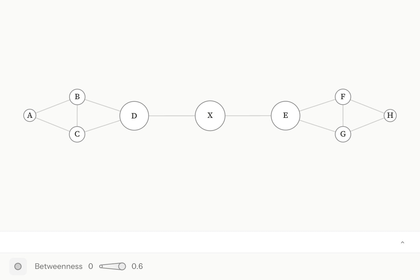
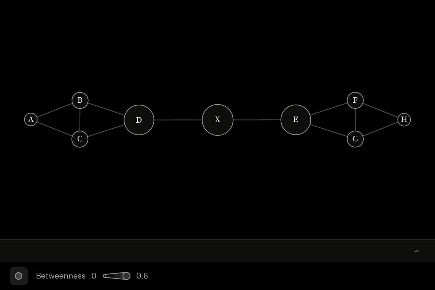
@data#pairs{
    a | b
    A | B
    A | C
    B | C
    C | D
    B | D
    E | F
    E | G
    F | G
    G | H
    F | H
    D | X
    X | E
}

network{
    vertices(size: #self.betweenness -> 0..0.6 -> 1 + 1.5_)
    edges(from: #pairs.a; to: #pairs.b)
}#Paths and walks
path is the shortest route through the vertices through names, in turn: path(through: #a, #f) from a to f, path(through: #a, #c, #f) from a to c and on to f. It counts weights where the network has them, follows direction on a directed network, and derives length and hops. It is drawn as a broad stroke over the edges it takes; under cue.draw the stroke draws along its route.
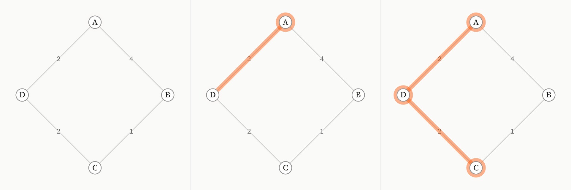
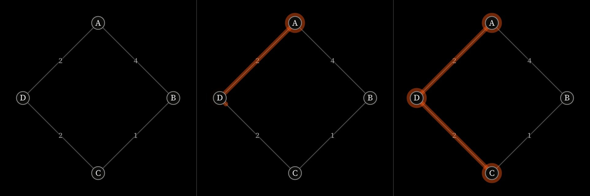
network:circle{
    vertex#a{A}
    vertex#b{B}
    vertex#c{C}
    vertex#d{D}
    edge(from: #a; to: #b; weight: 4)
    edge(from: #b; to: #c; weight: 1)
    edge(from: #a; to: #d; weight: 2)
    edge(from: #d; to: #c; weight: 2)

    cue.draw{
        path(through: #a, #c)
    }(
        in: 1
        in duration: 1.4s
    )
}(
    show weights
)
Where several routes are equally short, the path takes one of them, the same one every time, by no rule a reader can see. Where some leg has no route at all, as on a directed network with no way back or between two components, the path draws nothing and derives nothing, so prose citing its length reads as absent rather than as a wrong number.
through may name edges instead, by the ids inline edges declare, and then the path is the walk along them exactly as written: path(through: #e1, #e2, #e3). A list names vertices or edges, never both. A walk can take a self-loop, one of two parallel edges, or an edge twice, which no list of vertices can say, so an Eulerian path is written as a walk. Each edge must leave from where the one before it ended:
network{
    vertex#a{A}
    vertex#b{B}
    vertex#c{C}
    edge#e1(from: #a; to: #b)
    edge#e2(from: #b; to: #c)
    path(through: #e1, #e2)
}(
    directed: arrows
)
The same two edges in the other order are refused:
network{
    vertex#a{A}
    vertex#b{B}
    vertex#c{C}
    edge#e1(from: #a; to: #b)
    edge#e2(from: #b; to: #c)
    path(through: #e2, #e1)
}(
    directed: arrows
)[semantic]'path.through' cannot take '#e1' after '#e2' — each edge must leave from the vertex the one before it ended at, by its from: on a directed network
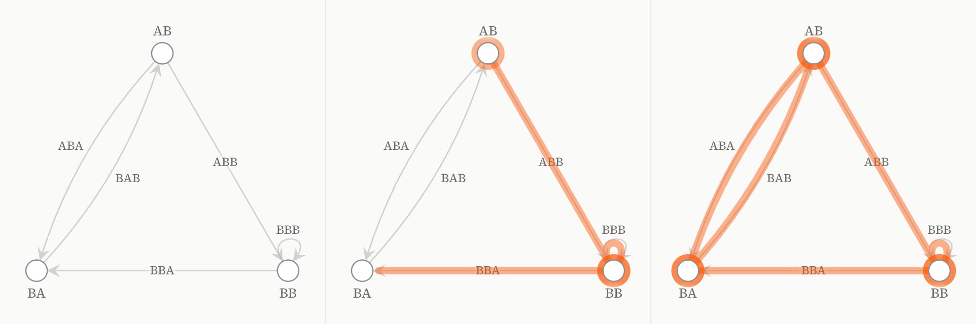
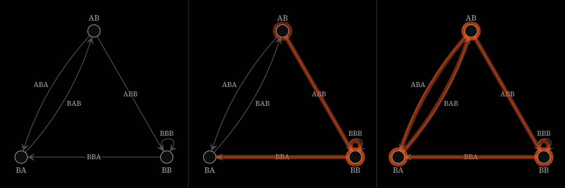
network:circle{
    vertex#ab{AB}
    vertex#bb{BB}
    vertex#ba{BA}
    edge#abb(from: #ab; to: #bb; label: ABB)
    edge#bbb(from: #bb; to: #bb; label: BBB)
    edge#bba(from: #bb; to: #ba; label: BBA)
    edge#bab(from: #ba; to: #ab; label: BAB)
    edge#aba(from: #ab; to: #ba; label: ABA)

    cue.draw{
        path(through: #abb, #bbb, #bba, #bab, #aba)
    }(
        in: 1
        in duration: 2s
    )
}(
    directed: arrows
)#focus and interactive
focus names what the camera looks at, and the camera finds the zoom from it, up to four times the fit. fit, the default, is the whole network. Ids of vertices or paths are framed together; a path by its route; a single vertex among its neighbours, since what a vertex connects to is what it means. A point of the frame, 0.62, 0.31, centres the fit there. It animates with !cue.to, the camera flying between the frames: focus: fit !cue.to{#hub}(at: 1; duration: 1.4s). Vertices keep their size as the frame closes in, so a dense neighbourhood pulls apart rather than magnifying the tangle. interactive hands the reader wheel-zoom and drag, with a double-click back to the authored frame.
#Attributes
layoutforcecirclegridtreebinary-treelayeredbipartitechordflownetwork:valueforcedirectedfrom to to, and how that is drawn.nonearrowscurvesnonedirectiondownrightdownroot#id of the vertex a tree, binary-tree or undirected layered layout starts from.network-refseed0show-weightslabel: with its weight.weightsfalselegendtruetitlefocusnetwork-focusfitinteractivefalsecontinue#Derived attributes
Computed while the element renders — read one with #id.name in attribute position or {{#id.name}} in prose, never set.
verticesedgescomponentscommunitiesdensitydiameter#Allowed content
#Allowed in
#Examples
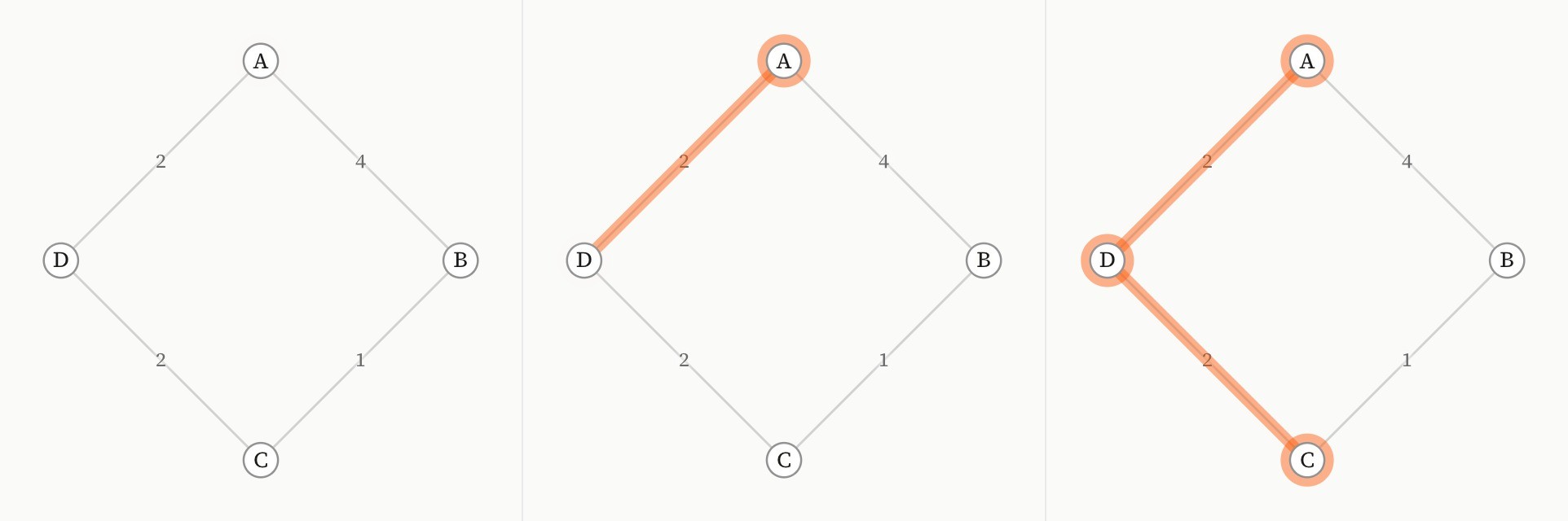
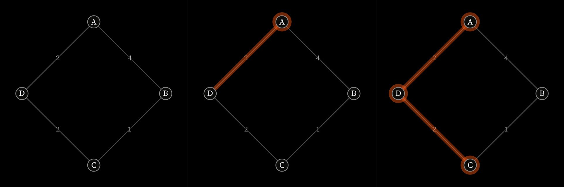
network:circle{
    vertex#a{A}
    vertex#b{B}
    vertex#c{C}
    vertex#d{D}
    edge(from: #a; to: #b; weight: 4)
    edge(from: #b; to: #c; weight: 1)
    edge(from: #a; to: #d; weight: 2)
    edge(from: #d; to: #c; weight: 2)
    cue.draw{
        path#route(through: #a, #c)
    }(
        in: 1
    )
}(
    show-weights: true
)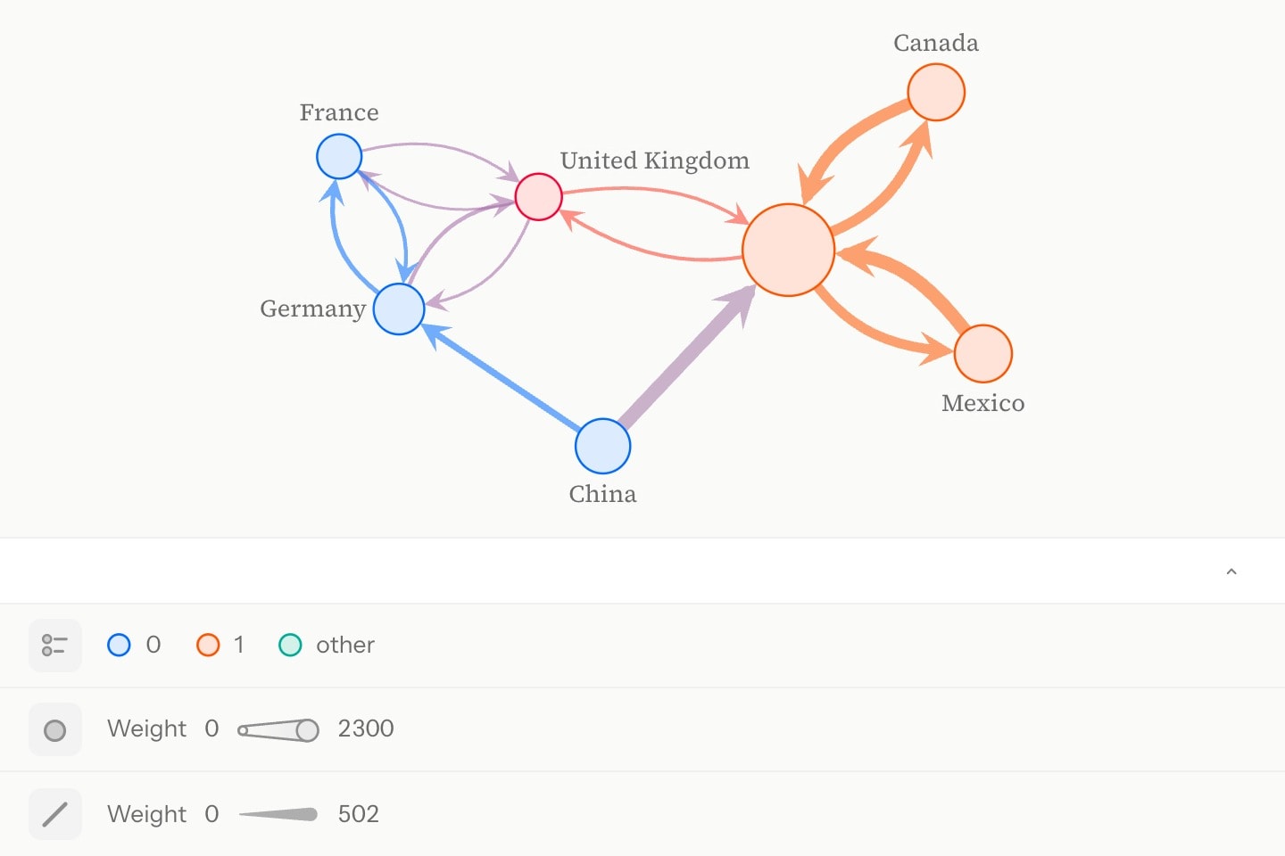
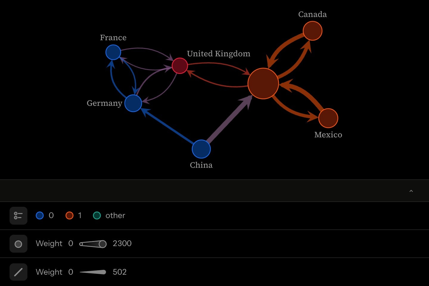
network{
    vertex#uk{United Kingdom}(colour: red)
    vertices(size: #self.weight -> 0..2300 -> 1 + 1.5_; colour: #self.community -> (0: blue; 1: orange; otherwise: teal))
    edges(from: #trade.exporter; to: #trade.importer; weights: #trade.value; width: #self.weight -> 0..502 -> 1 + 7_; colour-from: ends)
}(
    directed: arrows
)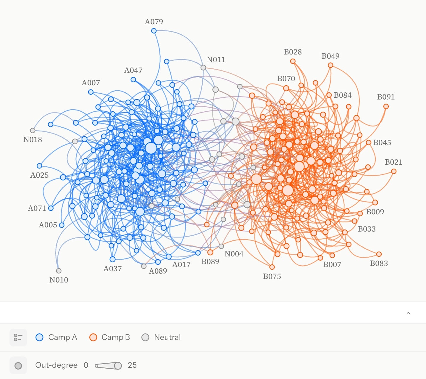
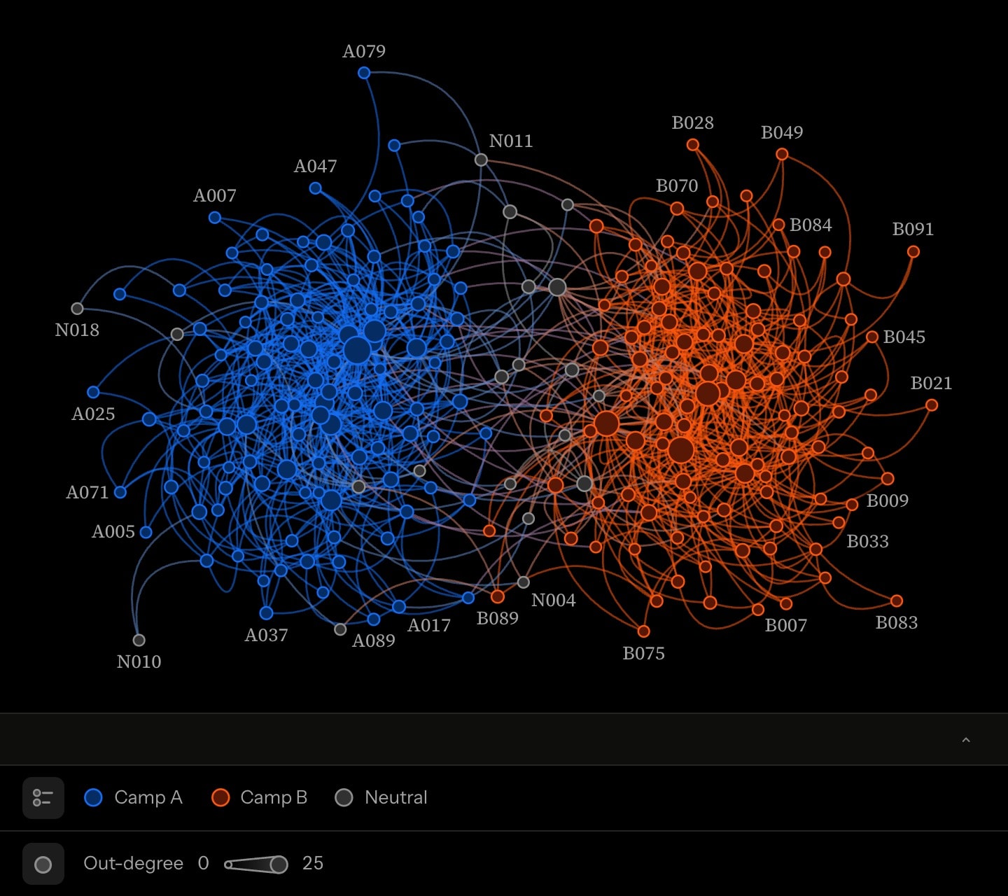
network{
    vertices(names: #accounts.handle; colour: #accounts.camp -> (Camp A: blue; Camp B: orange; Neutral: grey); size: #self.out-degree -> 0..25 -> 1 + 1.5_)
    edges(from: #retweets.original; to: #retweets.retweeter; colour-from: ends)
}(
    directed: curves
)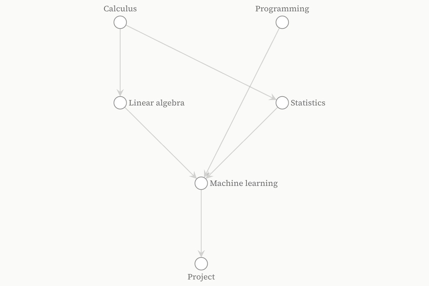
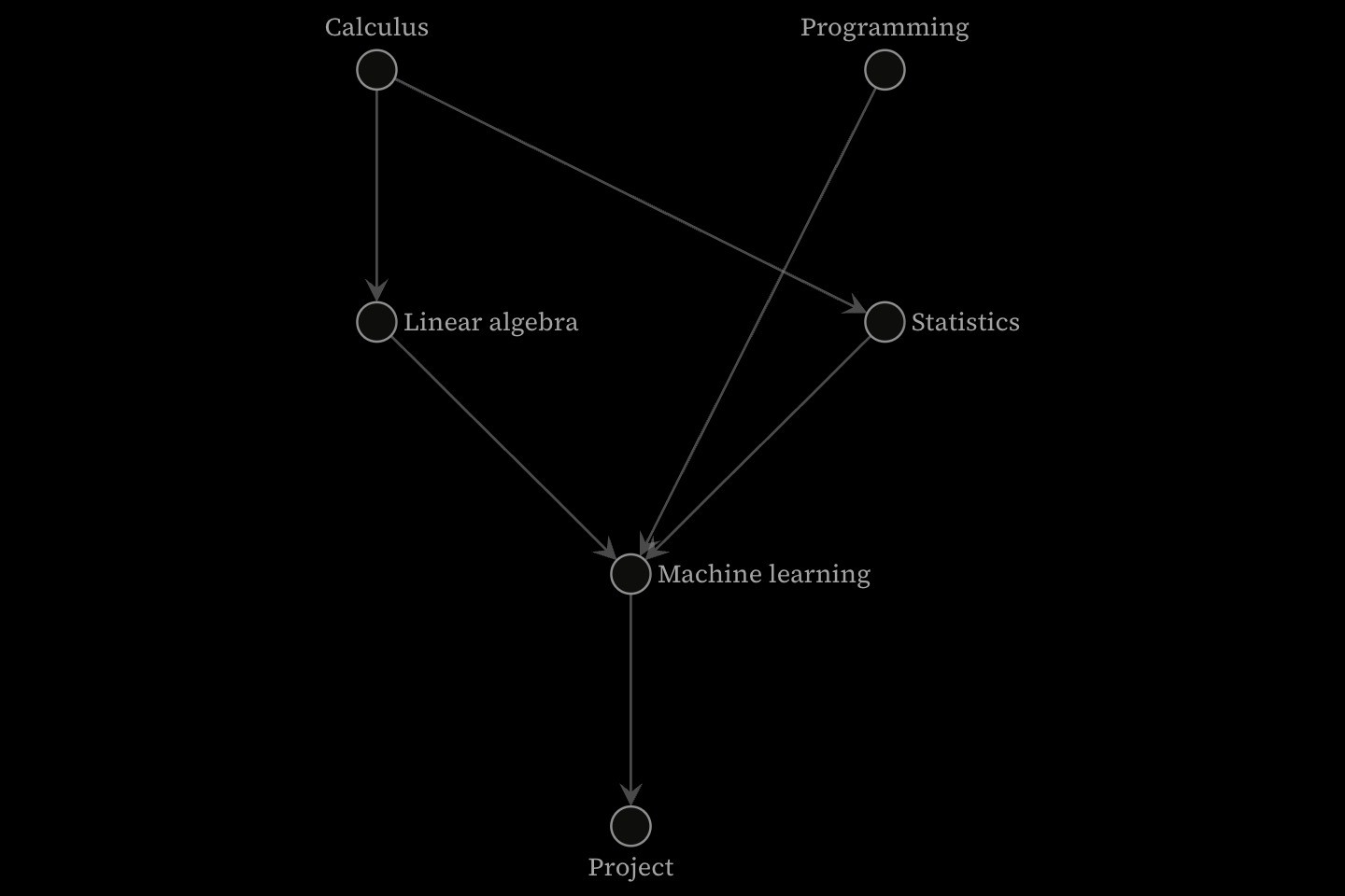
network:layered{
    vertex#calc{Calculus}
    vertex#prog{Programming}
    vertex#linalg{Linear algebra}
    vertex#stats{Statistics}
    vertex#ml{Machine learning}
    vertex#thesis{Project}
    edge(from: #calc; to: #linalg)
    edge(from: #calc; to: #stats)
    edge(from: #prog; to: #ml)
    edge(from: #linalg; to: #ml)
    edge(from: #stats; to: #ml)
    edge(from: #ml; to: #thesis)
}(
    directed: arrows
)#Writing guidance
- Selecting canvas content — A mark belongs on the canvas when seeing it changes what the reader understands, and the detail holds as a picture on its own.