geo
A geographic environment on the scene's canvas. Its in: names the boundary pack the environment is drawn over — geo:world is a world map on its own, with no child node needed — and every overlay inside it inherits that pack. The body holds those overlays: a choropleth joined to an dataset, marker points, great-circle arc routes, further region layers, and the parameters that drive them. The frame is a camera rather than a pair of domains — centre: (latitude first) and zoom: (web-map doubling levels) — and both are animatable with !cue.to, so one keyframe on each is a fly-to. The committed packs ship with the library and an attached .geojson travels with the document, so nothing is ever fetched from a tile server: a map renders offline, under both themes, and identically in ten years.
geo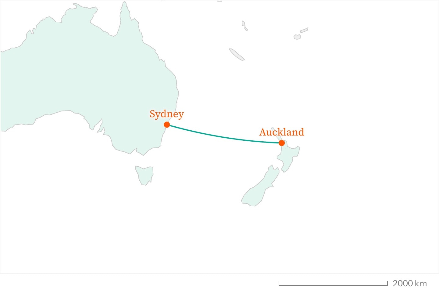
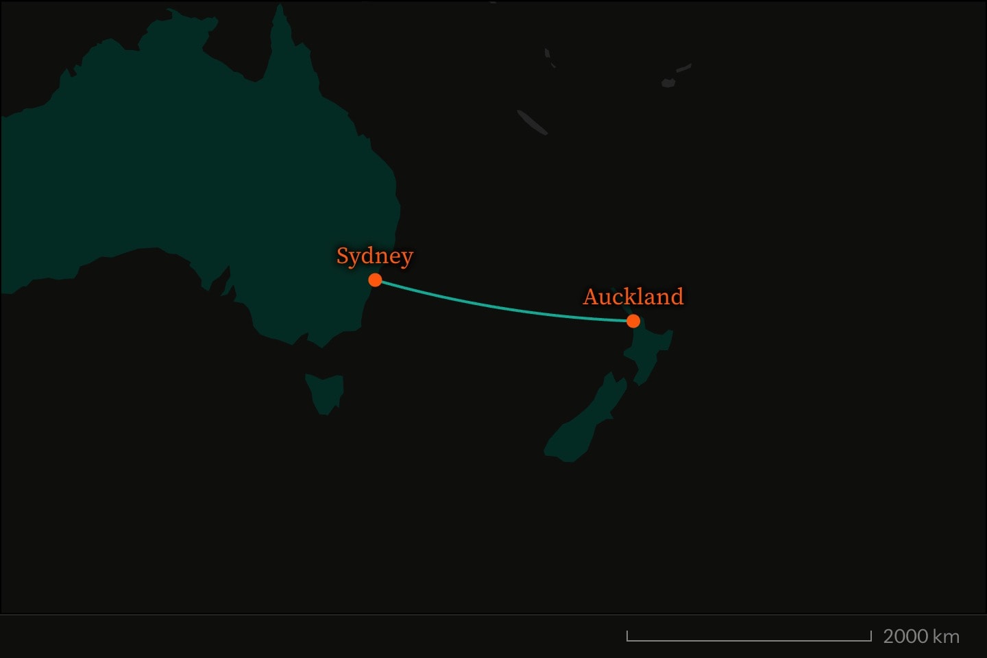
#The geographic environment
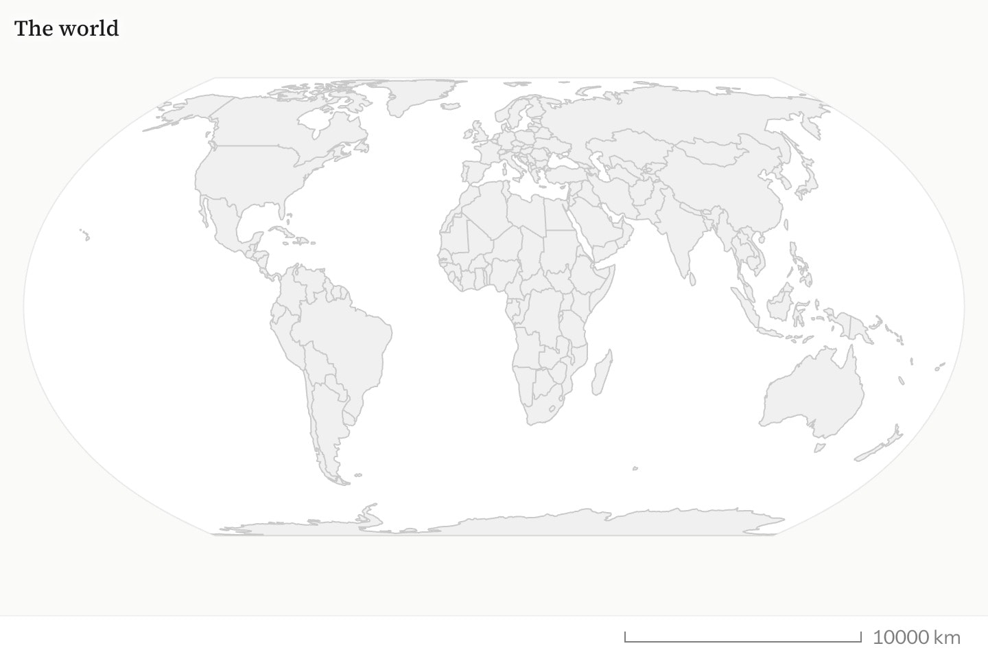
geo is a map surface. Its implicit attribute is in, the boundary pack the environment is drawn over, so geo:world{ } is already a world map with nothing inside it. The committed packs are world (Natural Earth 110m countries) and six admin-1 sets — us-states, canada-provinces, australia-states, uk-counties, nz-regions and europe-admin1. Every overlay in the body inherits that pack unless it names its own. title captions the environment, projection chooses how the sphere is laid flat, and show-scale (on by default) says what a length on screen is worth on the ground.
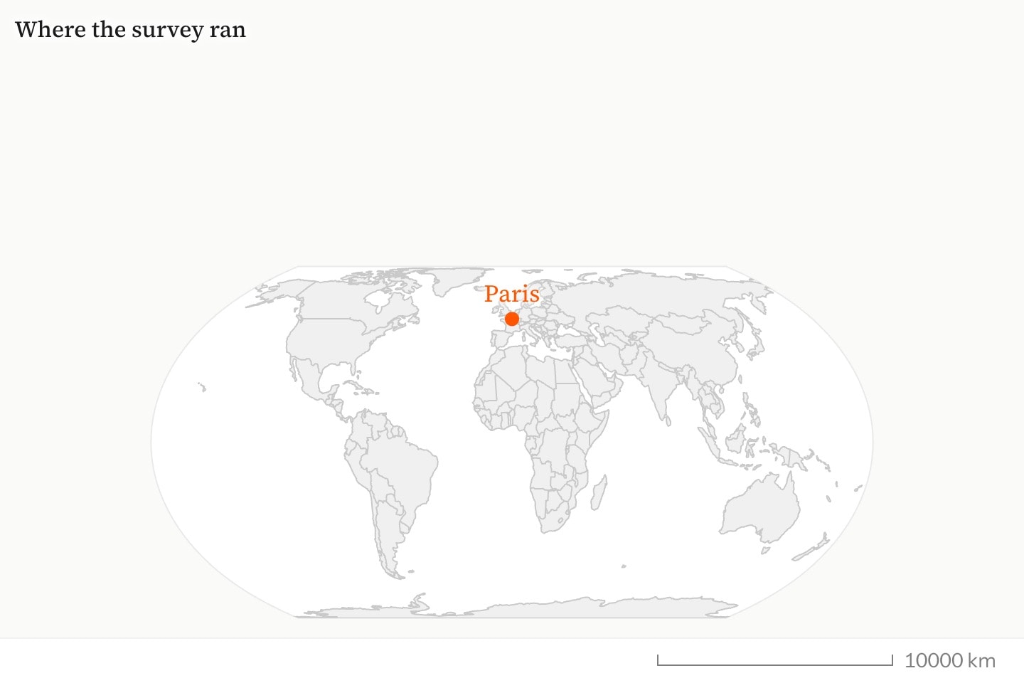
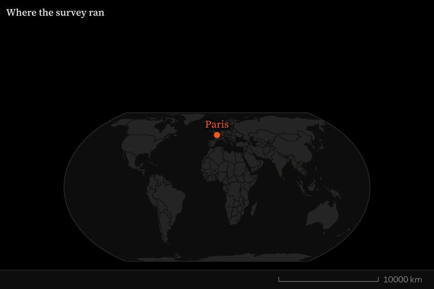
geo:world{
    marker(at: 48.85, 2.35; label: Paris)
}(
    title: Where the survey ran
    projection: equal-earth
)
Boundaries a pack does not carry — electorates, catchments, council wards — arrive as an attached .geojson file, and in names it the same way it names a pack: in: #wards, pointing at an declaration. Either way the geometry is drawn as SVG, exactly as a graph mark is, and nothing is fetched from a tile server — which is what lets a map render offline, under both themes, and identically in ten years.
equal-earth keeps areas honest and is the right world framing; mercator keeps angles honest and is the frame on which a great-circle route visibly bends; conic tunes its standard parallels to whatever the environment contains and is the right choice for one country; albers-usa carries Alaska and Hawaii in as insets; globe is the sphere itself, the far hemisphere behind the horizon. Choose the one whose distortion your claim can afford.#centre, zoom and the fly-to
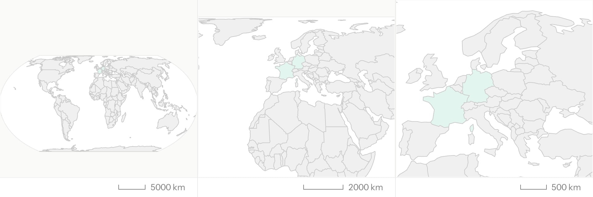
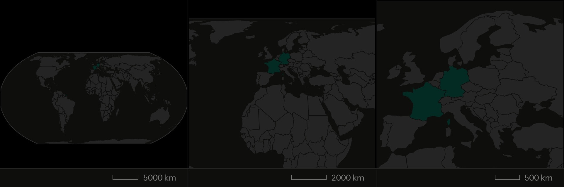
A geographic environment is framed by a camera rather than by a pair of domains: centre — latitude first — and zoom, in web-map doubling levels, where 1 fits the world's width and each level halves the span. Omit them both and the environment fits its own contents across the whole choreography, so a marker that travels stays framed at every point of its journey.
Both are animatable, and a !cue.to on each with the same anchor is the fly-to. A centre may also be written as #id naming a marker the environment already draws, so a map framed on Tokyo that also pins Tokyo states the place once; a keyframe onto a reference snaps rather than gliding, because a reference has no midpoint to interpolate through.
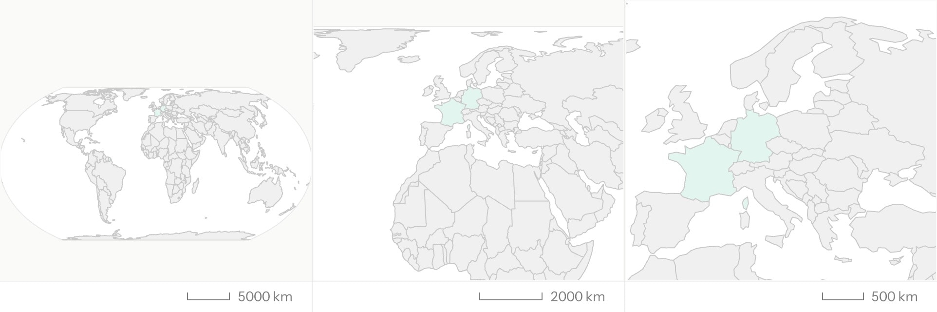
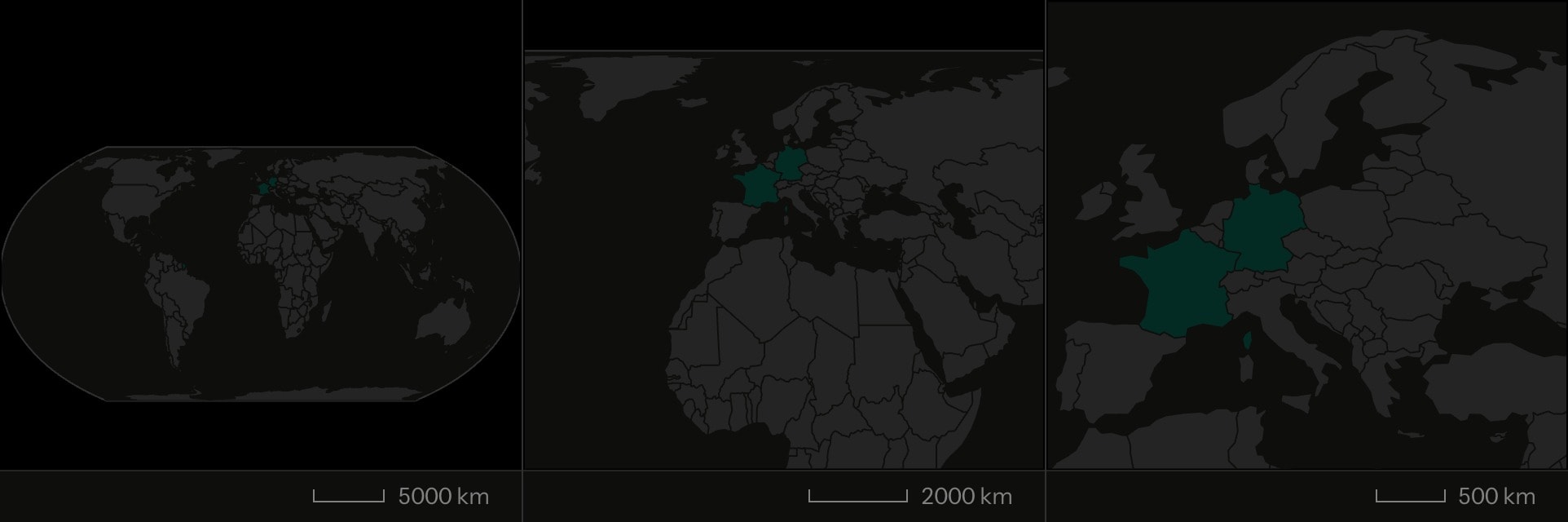
geo#tour:world{
    region(in: world; only: France, Germany; fill: teal)
}(
    centre: 20, 0 !cue.to{50.5, 15}(at: 1; over: 900ms)
    zoom: 1 !cue.to{4}(at: 1; over: 900ms)
)
interactive: true hands the camera to the reader — scroll to zoom, drag to pan, double-click to reset. Exploration stays on the environment's subject: the zoom floor is the frame that fits its packs, markers and arcs, so a reader cannot lose the map. Their camera then overrides the authored one for the session, and continue: #that-environment carries it into a later environment. The scene's parameters do not travel with it — they are not the map's to hand over.
#Overlays
Everything drawn over the basemap is an overlay, and the four share opacity and hidden (declared but not drawn, and animatable, so hidden: true !cue.to{false}(at: 2) is a reveal). Cues wrap overlays exactly as they wrap graph marks. The attention cues do not reach this environment: a highlight ring and a spotlight are plot machinery, and a geographic environment admits only cue and cue.draw.
#Boundary layers
The environment's in: already draws its pack, so a region is for what a basemap cannot say: a subset in its own colours, a second pack layered over the first, an attached.geojson over a committed pack, or boundaries that arrive on a cue. only and except narrow it by name or ISO alpha-3 code, matched case-insensitively — France, DEU and Ivory Coast all read — and fill, stroke and width paint what is left.
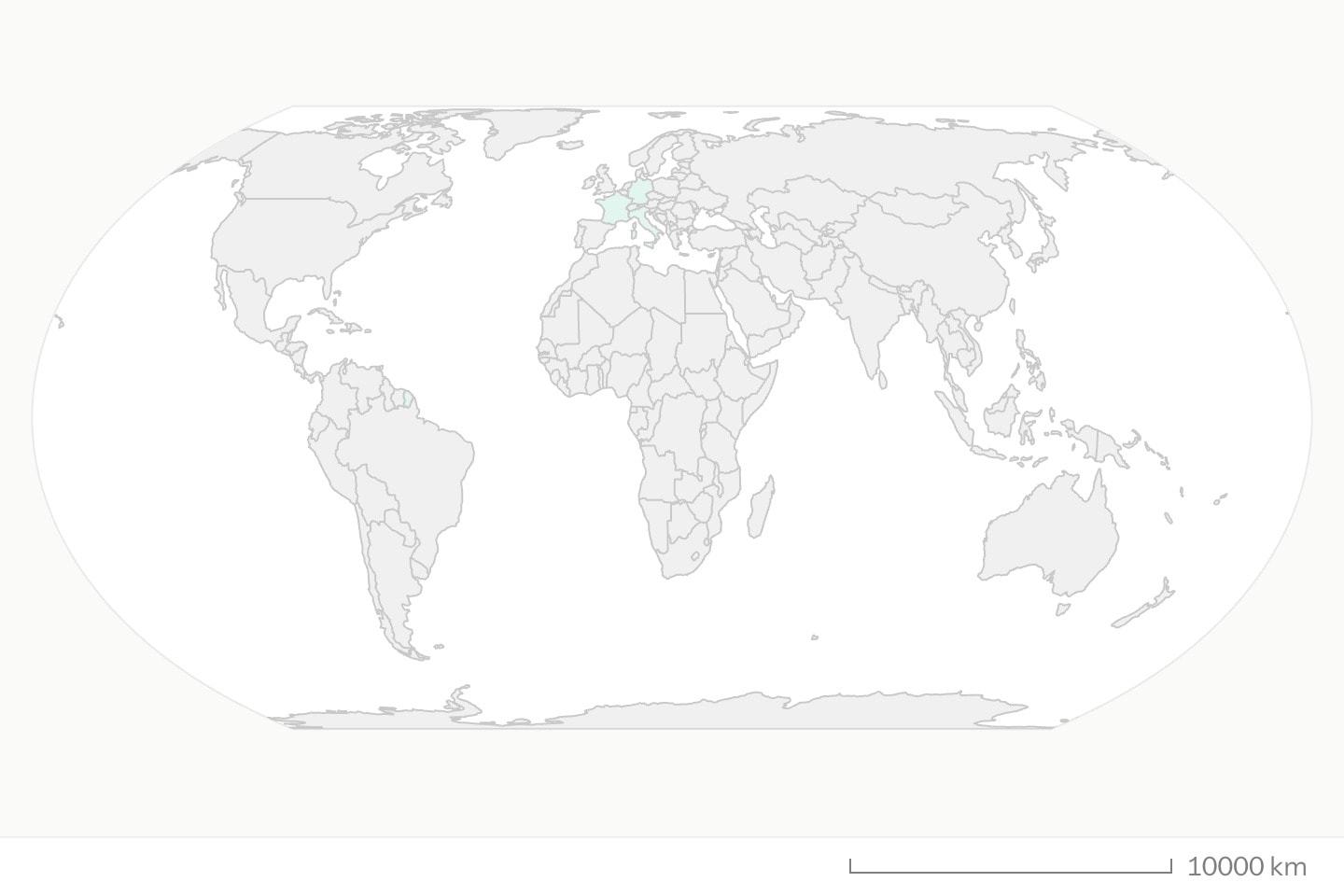
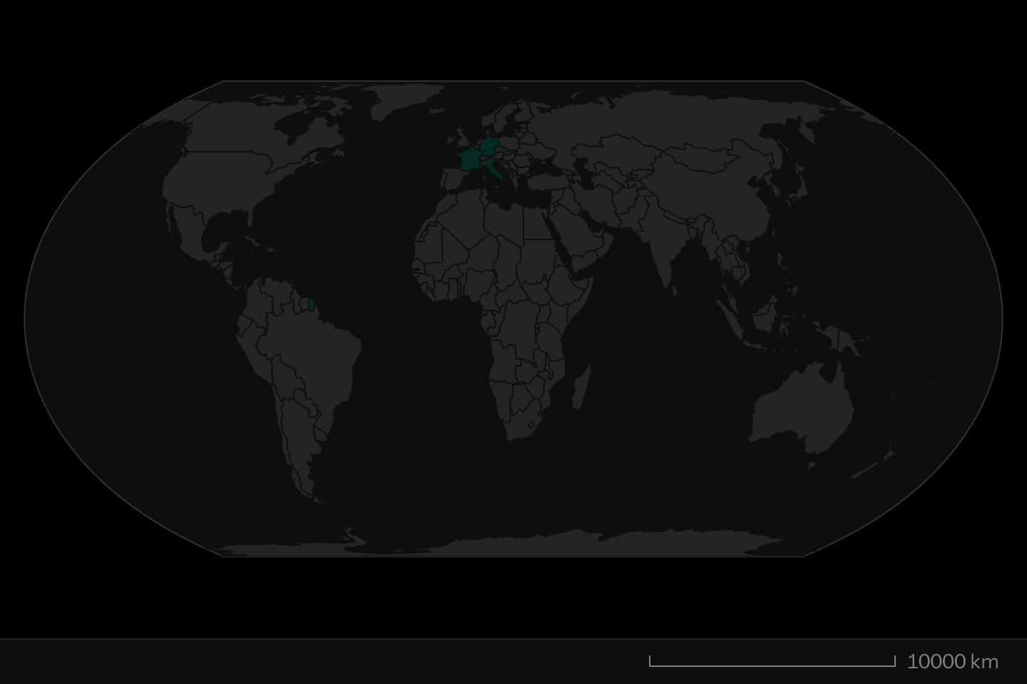
geo:world{
    region(in: world; except: Antarctica)
    region(in: world; only: France, Germany, Italy; fill: teal)
}#Joining a dataset to regions
choropleth joins a column onto the pack's regions — the geographic sibling of the graph's heatmap. regions names the column of region names and values the column to shade by; join keys match pack names and short codes case-insensitively, and a region the join does not cover keeps the neutral land fill rather than disappearing.
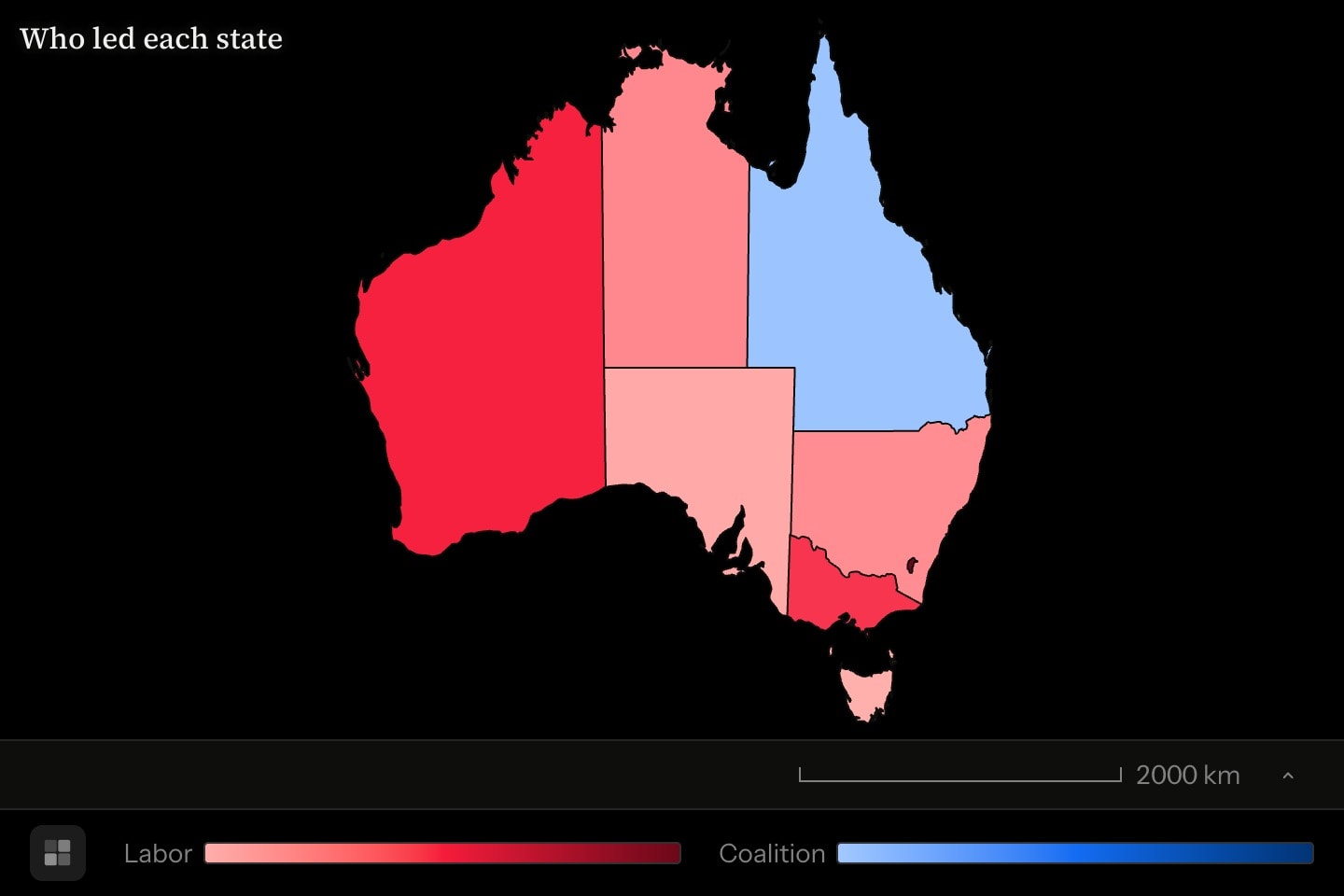
values is a column of numbers, always: where along a scale each region sits. Which scale is colour — multicolour, temperature, or a single hue's own intensity — with range pinning the window. Where one scale will not do, colours names a column of them, a cell per row holding whatever colour would; rows sharing a cell are one group in the legend and labels says what to call it. That is the electoral map's own grammar — the winner names the colour, the margin says how solid it is — and it is the same sentence as the single-scale map, with the scale varying by row rather than being one for all.
geo:australia-states{
    choropleth(
        regions: #vote.state
        values: #vote.margin
        colours: #vote.colour
        labels: #vote.party
    )
}(
    title: Who led each state
)min, max, mean and count over the values the join actually covered, so prose can cite the spread the shading spans instead of a number typed in beside it: give the mark an id — choropleth#gdp(…) — and read {{#gdp.max}}.#Places
marker is a point on the earth, in two forms. Singly, at takes a coordinate, latitude first, with an optional label; either half may be an expression of the scene's parameters, so a marker rides a slider or a keyframe. Data-bound, lat and lon name columns and the one node draws every row — add size-by and symbol area scales with that column, which is the proportional-symbol map.
geo:world{
    marker(lat: #quakes.lat; lon: #quakes.lon; size-by: #quakes.magnitude; colour: red; opacity: 0.6)
}#Great-circle routes
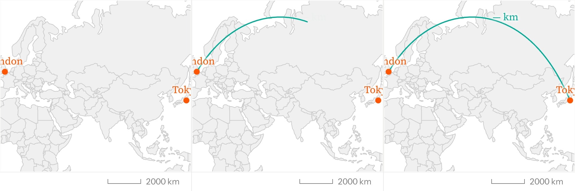
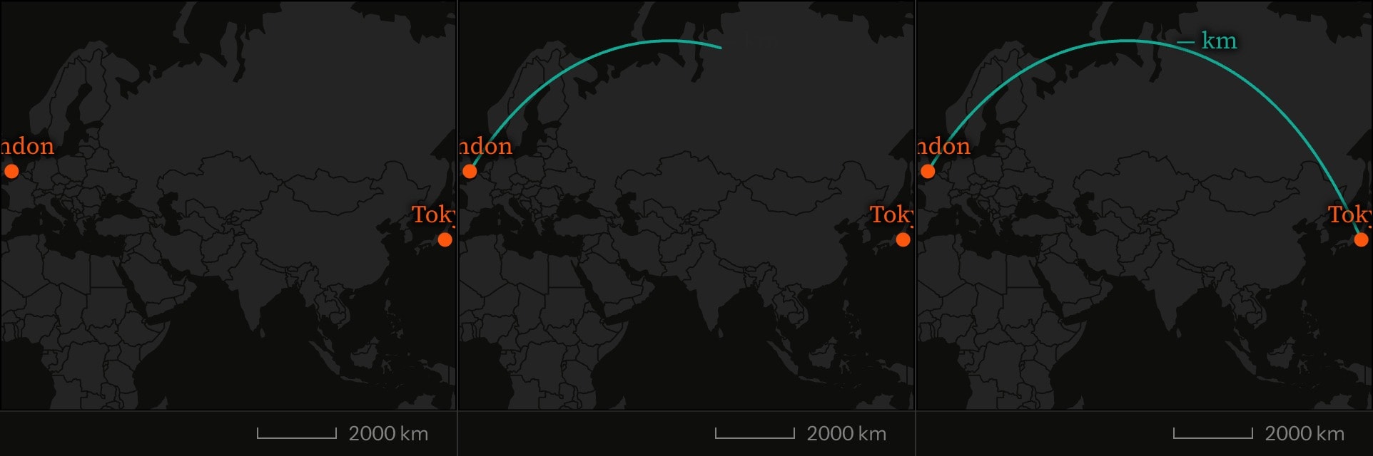
arc draws the great-circle path between two places — the shortest route over the earth, drawn the way the earth actually is. On a mercator environment the London–Tokyo arc bends far north of the straight line between them, and that one element is the whole projection-distortion lesson. Either end may be #id naming a marker in the same environment, and an anchored end follows its marker. An arc publishes derived distance in kilometres — the number the arc is.
geo:world{
    cue.draw{
        arc#route(from: #london; to: #tokyo; label: {{round(#route.distance, 0)}} km)
    }(
        in: 1
        in-duration: 1200ms
    )
    marker#london(at: 51.47, -0.46; label: London)
    marker#tokyo(at: 35.55, 139.78; label: Tokyo)
}(
    projection: mercator
)#Moving a map through time
A map moves through its data in one of two ways, and which one is a fact about the data. For a handful of slices, chain the columns: values is animatable, so #y1990.rate !cue.to{#y2000.rate}(at: 1) eases every region between its own two readings. Pin range when you do, or the ramp re-normalises each frame and the change erases itself.
For long-format data — one row per region per slice — a control bound over: the slice column is the better tool. It takes its range, its stops and its format from the data rather than being told them, so naming the column gives the scene a scrubber over exactly that span; marks carrying a slice: read themselves against it, interpolating between the two values that bracket wherever the reader is standing. Writing it as a cue.slider hands the scrubbing to the scene: the map runs its years from the anchor, and the step's own transport plays it.
geo:world{
    cue.slider#years:t(over: #rates.year; name: Year; at: 1; duration: 12s)
    choropleth(regions: #rates.country; values: #rates.rate; slice: #rates.year; range: [0, 220])
}
A slice column of NAMES rather than years works the same way and cannot be interpolated — there is nothing between Brazil and China — so the control for it is a selector, and the map shows the rows carrying the name the reader picked.
Parameters and cues gives the rule the choice actually turns on: a change belongs to a scrubber when one sentence holds across its whole range, and to a cue otherwise.
#Derived attributes
Two overlays compute something and publish it for reading: a choropleth's min, max, mean and count, and an arc's distance. A control publishes value, where its parameter is standing — the year, on one bound over: a column of them. A selector whose values are names publishes nothing, since a live value is a number. Reach one by member access on the node's id — #route.distance in an attribute, {{#route.distance}} in prose. Derived attributes covers how they behave.
#Attributes
inworld is Natural Earth 110m countries; the other six are admin-1 packs. It may instead be #id naming an attached .geojson dataset — in: #wards — which makes the attachment itself the boundaries. Normally written in the head, geo:world, the way code:python is.worldus-statescanada-provincesaustralia-statesuk-countiesnz-regionseurope-admin1basemapCan be written as shorthand: geo:valuenames.geojson only: the feature property holding each region's name, which is what a choropleth joins on. Absent, the first of name, NAME, title or id the features carry.codes.geojson only: a feature property holding a short join code — the custom equivalent of a pack region's ISO alpha-3.simplify.geojson only: Douglas–Peucker tolerance in degrees, thinning boundary detail as the file is read. 0 keeps every point; a large file wants about 0.01.0titletitle: this one is visible content and not merely an accessible name. Rich text, so $maths$ and inline formatting render.projectionequal-earth, the default, keeps AREAS honest and is the right world framing. mercator keeps ANGLES honest: the frame every slippy map uses, and the one on which a great-circle arc visibly bends away from the straight line. equirectangular plots latitude and longitude straight. conic is an Albers equal-area conic that tunes its standard parallels to whatever the environment contains — what national atlases use, and the right choice for a single country or region. albers-usa is the United States composite, the lower 48 on an equal-area conic with Alaska and Hawaii carried in as insets, so a US environment spends no width on the Pacific. globe is the sphere itself, orthographic, with the far hemisphere behind the horizon.equal-earthmercatorequirectangularconicalbers-usaglobeequal-earthcentrecentre: 48.85, 2.35 — or #id naming a marker this environment already draws, centre: #tokyo, so the place is stated once. Either half of a coordinate may be a parametised expression. Animatable: centre: 20, 0 !cue.to{50.5, 15}(at: 2; over: 900ms) pans the frame, and writing the same anchor on zoom: makes the two move as one fly-to. A keyframe targeting a #id snaps rather than gliding, because a reference has no midpoint to interpolate through. Omitted, the environment frames its own contents.centerzoomlevels: 1 fits the world's width, and each level halves the span. Omitted, the zoom is AUTOMATIC — the environment fits what is inside it across the whole choreography, so a marker that travels stays framed at every point of its journey; writing zoom: 1 asks for exactly 1 instead. Parametised, and animatable with !cue.to.interactivefalseshow-scalescaletrueshow-graticulegraticulefalsegraticule-spacingshow-graticule:.15continuecontinue: #that-environment. The reader's explored camera and their parameter values carry forward; every authored attribute is the new environment's own.#Allowed content
#Allowed in
#Examples
geo:world(title: The world)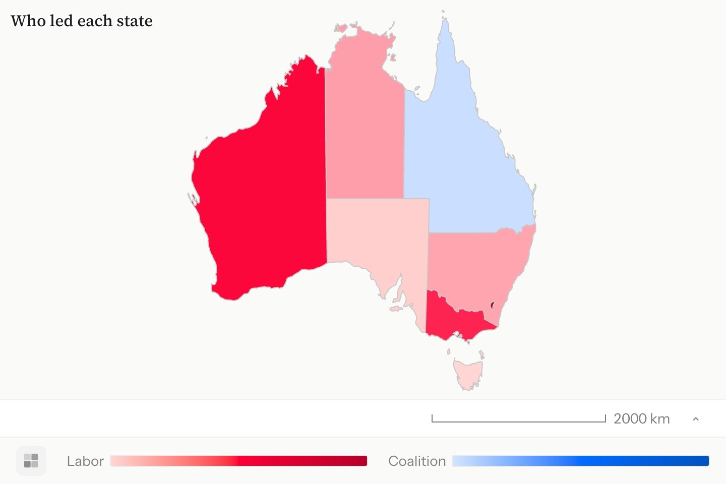
geo:australia-states{
    choropleth(regions: #vote.state; values: #vote.margin; colours: #vote.colour; labels: #vote.party)
}(
    title: Who led each state
)
geo#tour:world{
    region(in: world; only: France, Germany; fill: teal)
}(
    centre: 20, 0 !cue.to{50.5, 15}(at: 1; over: 900ms)
    zoom: 1 !cue.to{4}(at: 1; over: 900ms)
)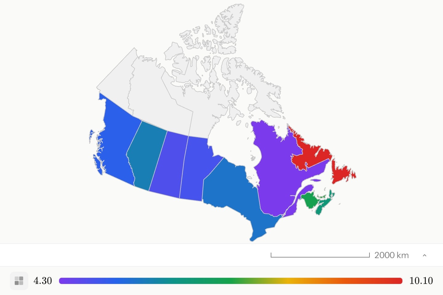
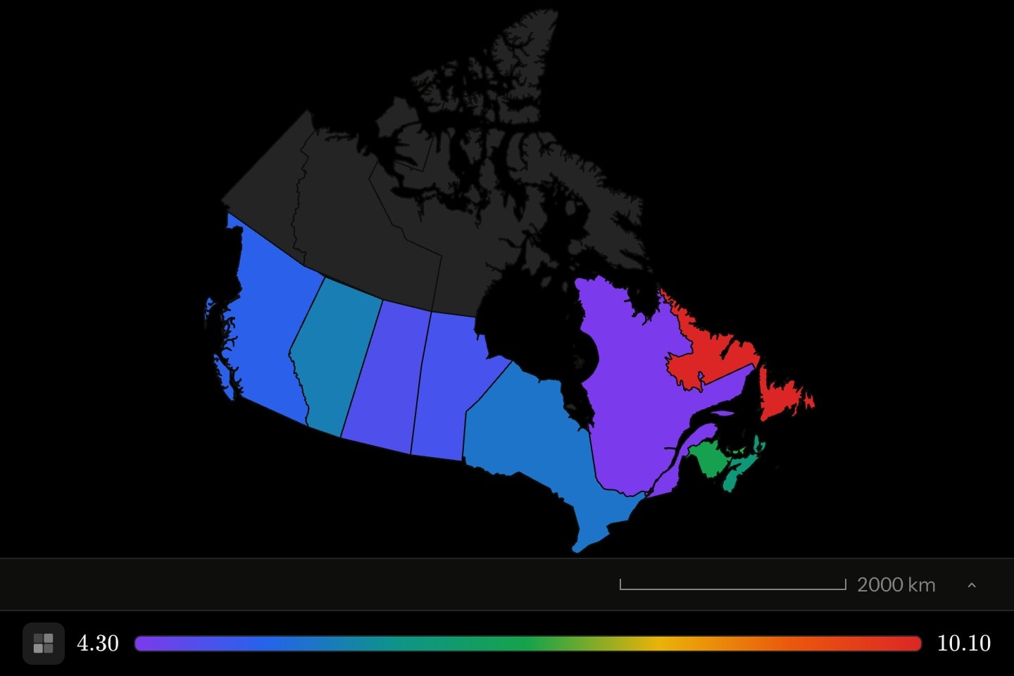
geo:canada-provinces{
    choropleth(regions: #d.province; values: #d.rate)
}(
    projection: conic
)#Notes
- An environment's own id is written on the node —
geo#europe{…}— andcontinue:points back at it with#europe. - Cues wrap overlays exactly as they wrap graph marks, and
cue.drawtraces anarcalong its length. - The cursor's coordinates, and the name of the region beneath it, read out in the corner of the environment.