biology
Import it with :biology, then call its constructs under that name.
@use:biology#Constructs
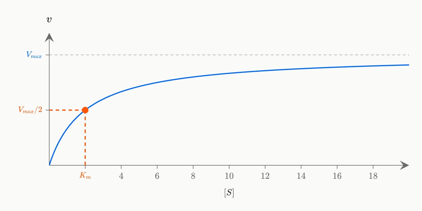
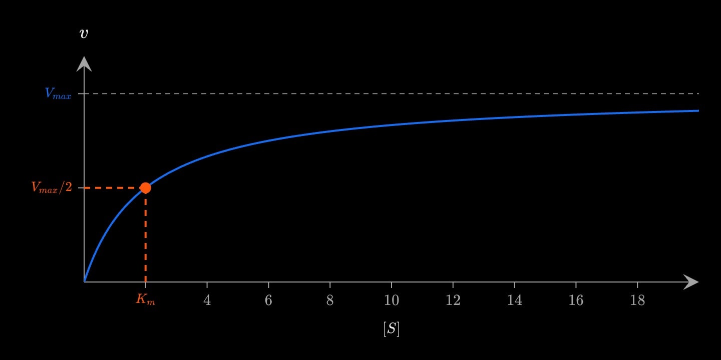
biology.michaelis-mentenThe Michaelis–Menten curve : the rate rising towards , ruled across the plot, with marked where the rate is half of it.
vmaxThe maximum rate the curve approaches, .
Default
10kmThe Michaelis constant : the substrate concentration at half the maximum rate.
Default
2smaxThe substrate concentration the curve is drawn out to.
Default
20labelThe curve's label.
inlineDefault
vmax-labelThe label on the ruled line at the maximum rate.
inlineDefault
$V_{max}$half-labelThe label on the rate axis at half the maximum.
inlineDefault
$V_{max}/2$km-labelThe label on the concentration axis at .
inlineDefault
$K_m$colourThe curve and the maximum rate's colour.
bluelight-bluedark-blueredlight-reddark-redorangelight-orangedark-orangeyellowlight-yellowdark-yellowteallight-tealdark-tealgreenlight-greendark-greenpinklight-pinkdark-pinkpurplelight-purpledark-purplegreylight-greydark-greyneutralhex(…)rgb(…)Default
bluemarker-colourThe half-maximum point and its dashed segments' colour.
bluelight-bluedark-blueredlight-reddark-redorangelight-orangedark-orangeyellowlight-yellowdark-yellowteallight-tealdark-tealgreenlight-greendark-greenpinklight-pinkdark-pinkpurplelight-purpledark-purplegreylight-greydark-greyneutralhex(…)rgb(…)Default
orangebiology.lineweaver-burkThe Lineweaver–Burk plot: Michaelis–Menten inverted, so the curve becomes the straight line . Across is and up is . The line is drawn back past the rate axis to meet the concentration axis at , and crosses the rate axis at .
![A blue straight Lineweaver–Burk line of 1/v against 1/[S], crossing the 1/v axis at 1/Vmax = 0.1 and drawn back to meet the 1/[S] axis at −1/Km = −0.5, both intercepts marked in orange.](/_next/image?url=%2Fmanual-figures%2Fhero-biology-lineweaver-burk.light.jpg&w=3840&q=90)
![A blue straight Lineweaver–Burk line of 1/v against 1/[S], crossing the 1/v axis at 1/Vmax = 0.1 and drawn back to meet the 1/[S] axis at −1/Km = −0.5, both intercepts marked in orange.](/_next/image?url=%2Fmanual-figures%2Fhero-biology-lineweaver-burk.dark.jpg&w=3840&q=90)
vmaxThe maximum rate, .
Default
10kmThe Michaelis constant, .
Default
2xmaxThe largest the line is drawn out to.
Default
2labelThe line's label.
inlineDefault
vmax-labelThe rate-axis intercept's label.
inlineDefault
$1/V_{max}$km-labelThe concentration-axis intercept's label.
inlineDefault
$-1/K_m$colourThe line's colour.
bluelight-bluedark-blueredlight-reddark-redorangelight-orangedark-orangeyellowlight-yellowdark-yellowteallight-tealdark-tealgreenlight-greendark-greenpinklight-pinkdark-pinkpurplelight-purpledark-purplegreylight-greydark-greyneutralhex(…)rgb(…)Default
bluemarker-colourThe two intercepts' colour.
bluelight-bluedark-blueredlight-reddark-redorangelight-orangedark-orangeyellowlight-yellowdark-yellowteallight-tealdark-tealgreenlight-greendark-greenpinklight-pinkdark-pinkpurplelight-purpledark-purplegreylight-greydark-greyneutralhex(…)rgb(…)Default
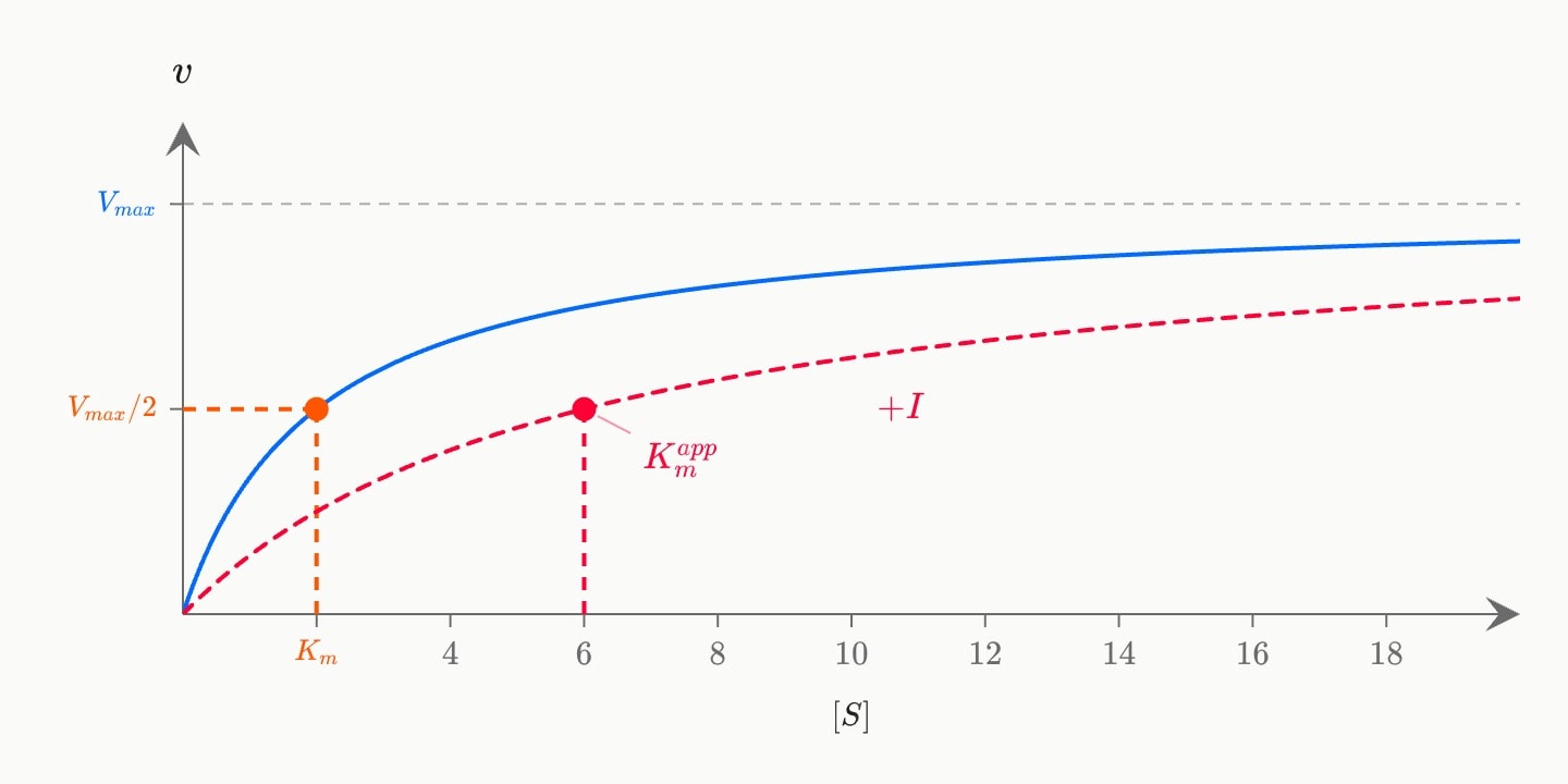
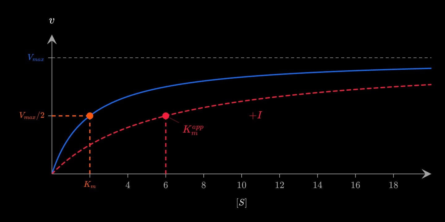
orangebiology.competitive-inhibitionA competitive inhibitor, drawn dashed over the uninhibited curve: the inhibitor competes for the active site, so the apparent rises to while is unchanged — enough substrate still outcompetes it.
vmaxThe uninhibited maximum rate, .
Default
10kmThe uninhibited Michaelis constant, .
Default
2inhibitorThe inhibitor's concentration, .
Default
2kiThe inhibitor's dissociation constant, .
Default
1smaxThe substrate concentration the curve is drawn out to.
Default
20labelThe inhibited curve's label.
inlineDefault
$+I$point-labelThe apparent 's label.
inlineDefault
$K_m^{app}$colourThe inhibited curve and its half-maximum point's colour.
bluelight-bluedark-blueredlight-reddark-redorangelight-orangedark-orangeyellowlight-yellowdark-yellowteallight-tealdark-tealgreenlight-greendark-greenpinklight-pinkdark-pinkpurplelight-purpledark-purplegreylight-greydark-greyneutralhex(…)rgb(…)Default
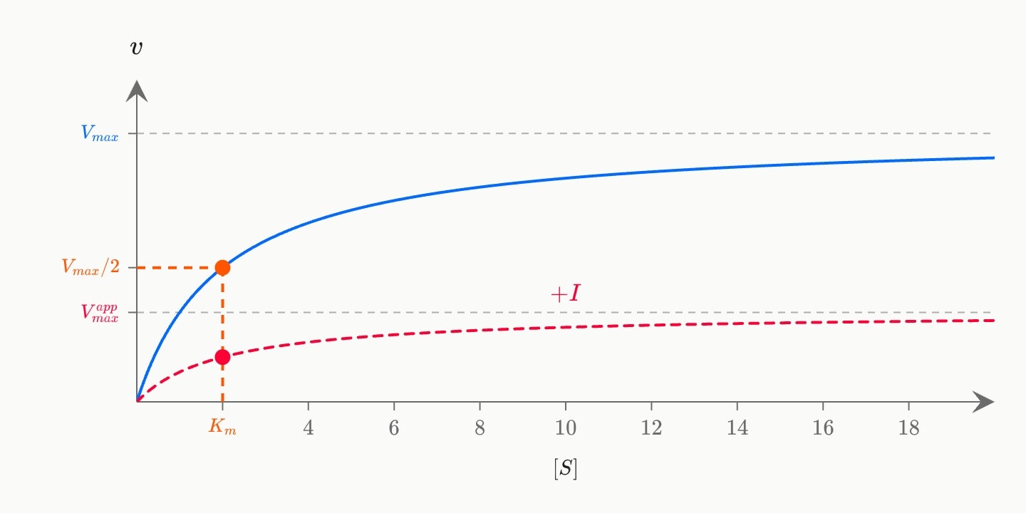
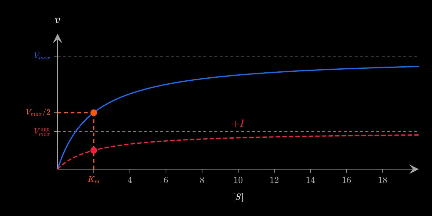
redbiology.noncompetitive-inhibitionA noncompetitive inhibitor, drawn dashed over the uninhibited curve: the inhibitor binds away from the active site, so the apparent falls to while is unchanged — the half-maximum point stays above the same concentration.
vmaxThe uninhibited maximum rate, .
Default
10kmThe Michaelis constant, , which the inhibitor leaves alone.
Default
2inhibitorThe inhibitor's concentration, .
Default
2kiThe inhibitor's dissociation constant, .
Default
1smaxThe substrate concentration the curve is drawn out to.
Default
20labelThe inhibited curve's label.
inlineDefault
$+I$vmax-labelThe label on the ruled line at the apparent maximum rate.
inlineDefault
$V_{max}^{app}$colourThe inhibited curve, its ruled maximum and its half-maximum point's colour.
bluelight-bluedark-blueredlight-reddark-redorangelight-orangedark-orangeyellowlight-yellowdark-yellowteallight-tealdark-tealgreenlight-greendark-greenpinklight-pinkdark-pinkpurplelight-purpledark-purplegreylight-greydark-greyneutralhex(…)rgb(…)Default
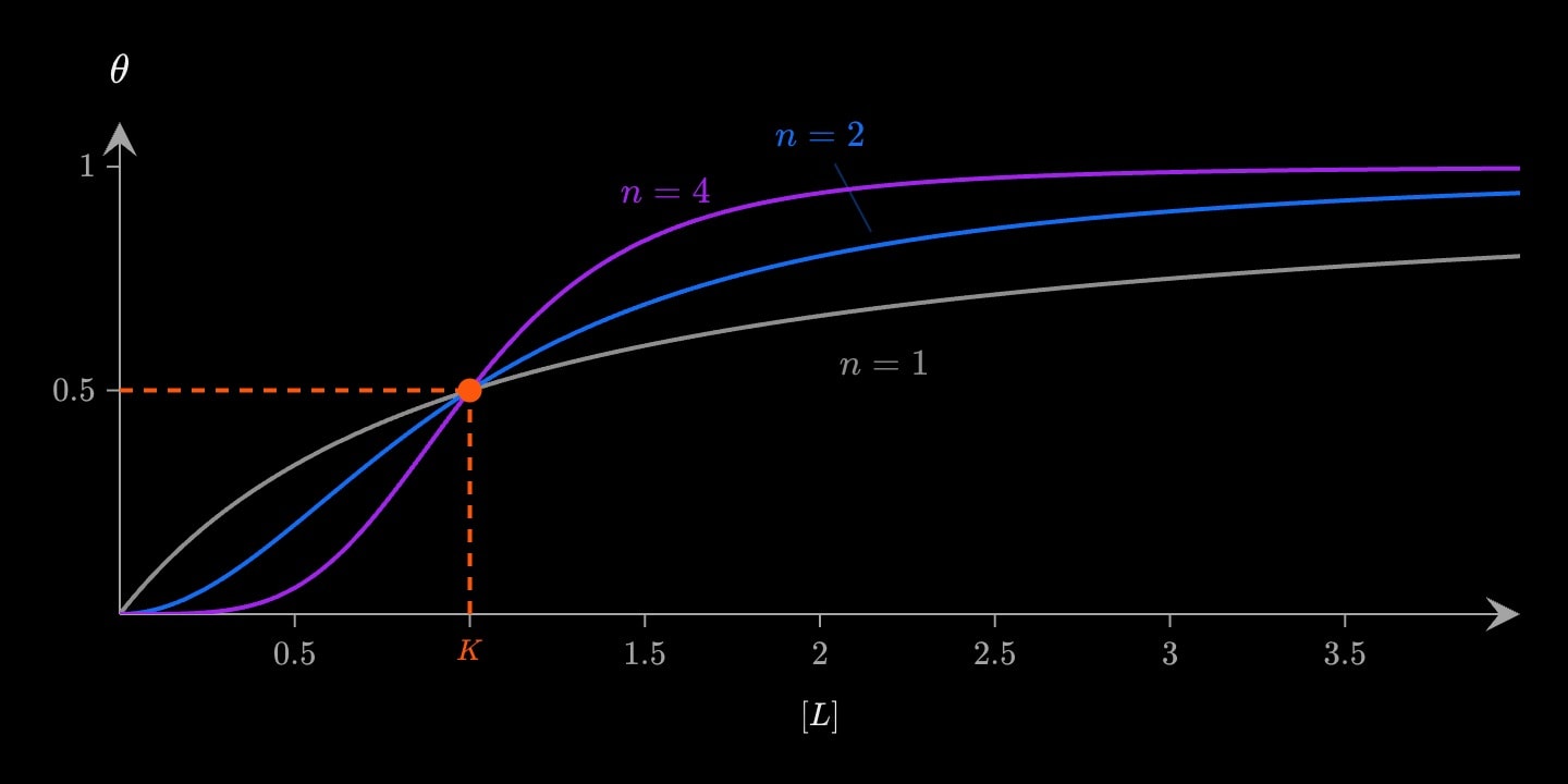
redbiology.hillThe Hill equation : the fraction of sites bound, against ligand concentration. is a hyperbola; above 1 the binding is cooperative and the curve turns sigmoid. Every curve passes through half saturation at , which
marked drops to both axes.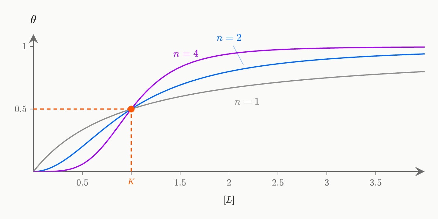
nThe Hill coefficient .
Default
2kThe ligand concentration at half saturation, .
Default
1lmaxThe ligand concentration the curve is drawn out to.
Default
4markedDrop half saturation to both axes. Several curves with one share the point, so mark it on one of them.
boolDefault
truek-labelThe label on the concentration axis at .
inlineDefault
$K$colourThe curve's colour.
bluelight-bluedark-blueredlight-reddark-redorangelight-orangedark-orangeyellowlight-yellowdark-yellowteallight-tealdark-tealgreenlight-greendark-greenpinklight-pinkdark-pinkpurplelight-purpledark-purplegreylight-greydark-greyneutralhex(…)rgb(…)Default
bluemarker-colourThe half-saturation point and its dashed segments' colour.
bluelight-bluedark-blueredlight-reddark-redorangelight-orangedark-orangeyellowlight-yellowdark-yellowteallight-tealdark-tealgreenlight-greendark-greenpinklight-pinkdark-pinkpurplelight-purpledark-purplegreylight-greydark-greyneutralhex(…)rgb(…)Default
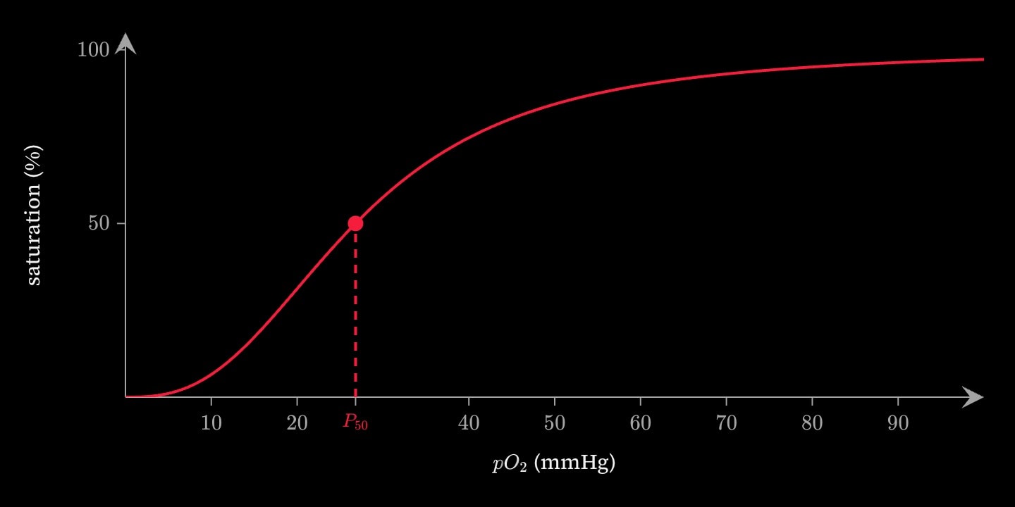
orangebiology.oxygen-dissociationHaemoglobin's oxygen dissociation curve: percentage saturation against the partial pressure of oxygen, a Hill curve with — the pressure at half saturation — dropped to the pressure axis. The defaults are adult human haemoglobin, in mmHg.
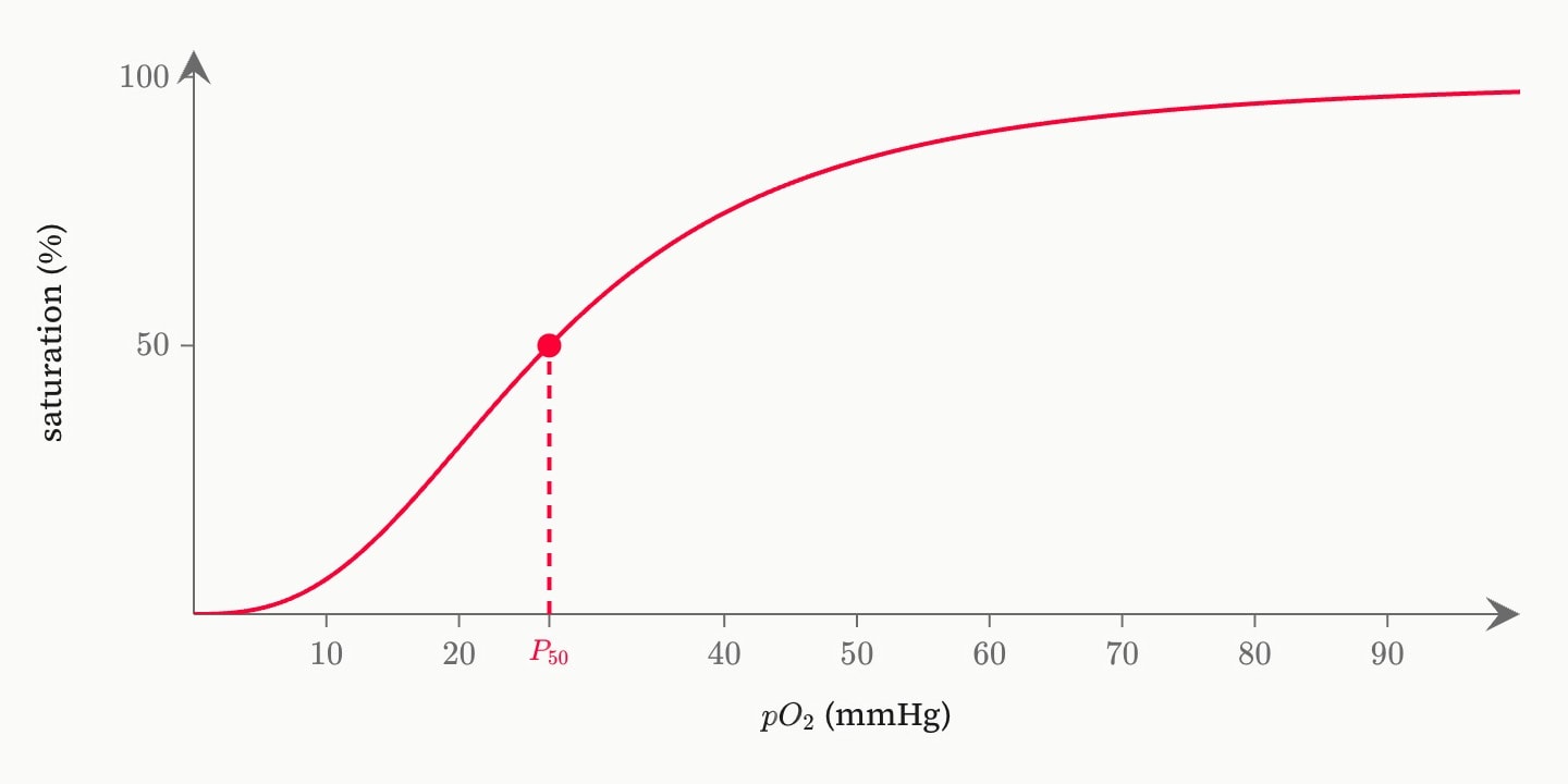
p50The partial pressure at half saturation, .
Default
26.8nThe Hill coefficient, how sigmoid the curve is.
Default
2.7pmaxThe partial pressure the curve is drawn out to.
Default
100labelThe curve's label.
inlineDefault
p50-labelThe label on the pressure axis at .
inlineDefault
$P_{50}$colourThe curve, its point and dashed segment's colour.
bluelight-bluedark-blueredlight-reddark-redorangelight-orangedark-orangeyellowlight-yellowdark-yellowteallight-tealdark-tealgreenlight-greendark-greenpinklight-pinkdark-pinkpurplelight-purpledark-purplegreylight-greydark-greyneutralhex(…)rgb(…)Default
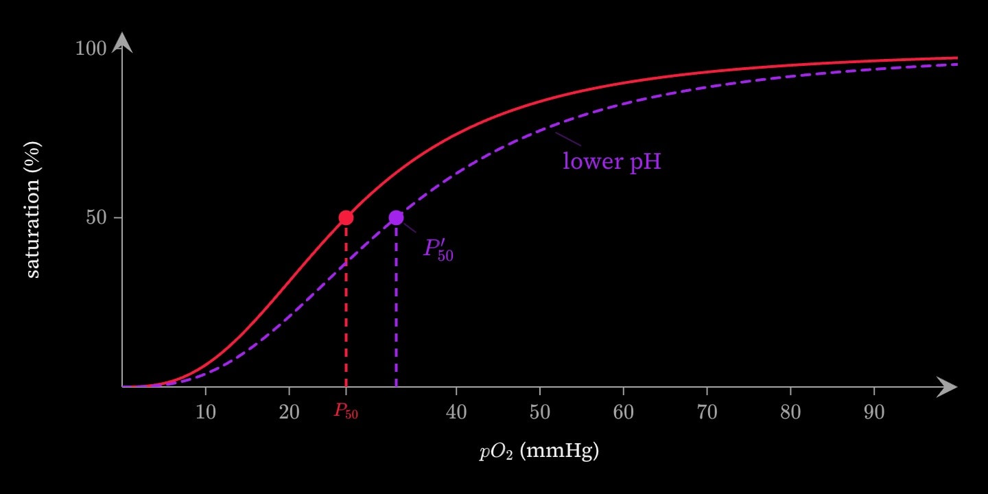
redbiology.bohr-shiftThe Bohr shift, drawn dashed over
oxygen-dissociation: lower pH or more carbon dioxide moves the curve right by by, so haemoglobin gives up more of its oxygen at the same pressure.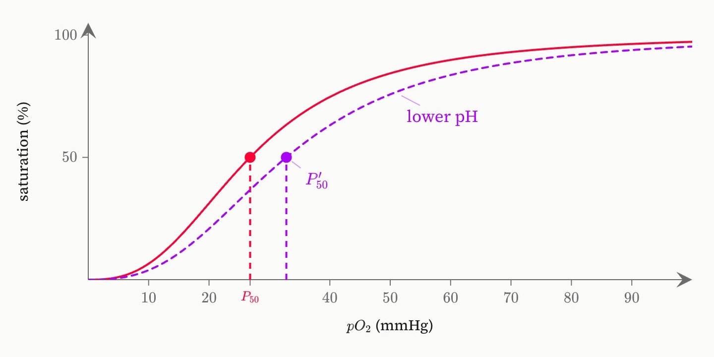
p50The original , as given to
oxygen-dissociation.Default
26.8nThe original Hill coefficient.
Default
2.7byHow far right the curve moves along the pressure axis.
Default
6pmaxThe partial pressure the curve is drawn out to.
Default
100labelThe shifted curve's label.
inlineDefault
lower pHpoint-labelThe shifted point's label.
inlineDefault
$P_{50}'$colourThe shifted curve, its point and dashed segment's colour.
bluelight-bluedark-blueredlight-reddark-redorangelight-orangedark-orangeyellowlight-yellowdark-yellowteallight-tealdark-tealgreenlight-greendark-greenpinklight-pinkdark-pinkpurplelight-purpledark-purplegreylight-greydark-greyneutralhex(…)rgb(…)Default
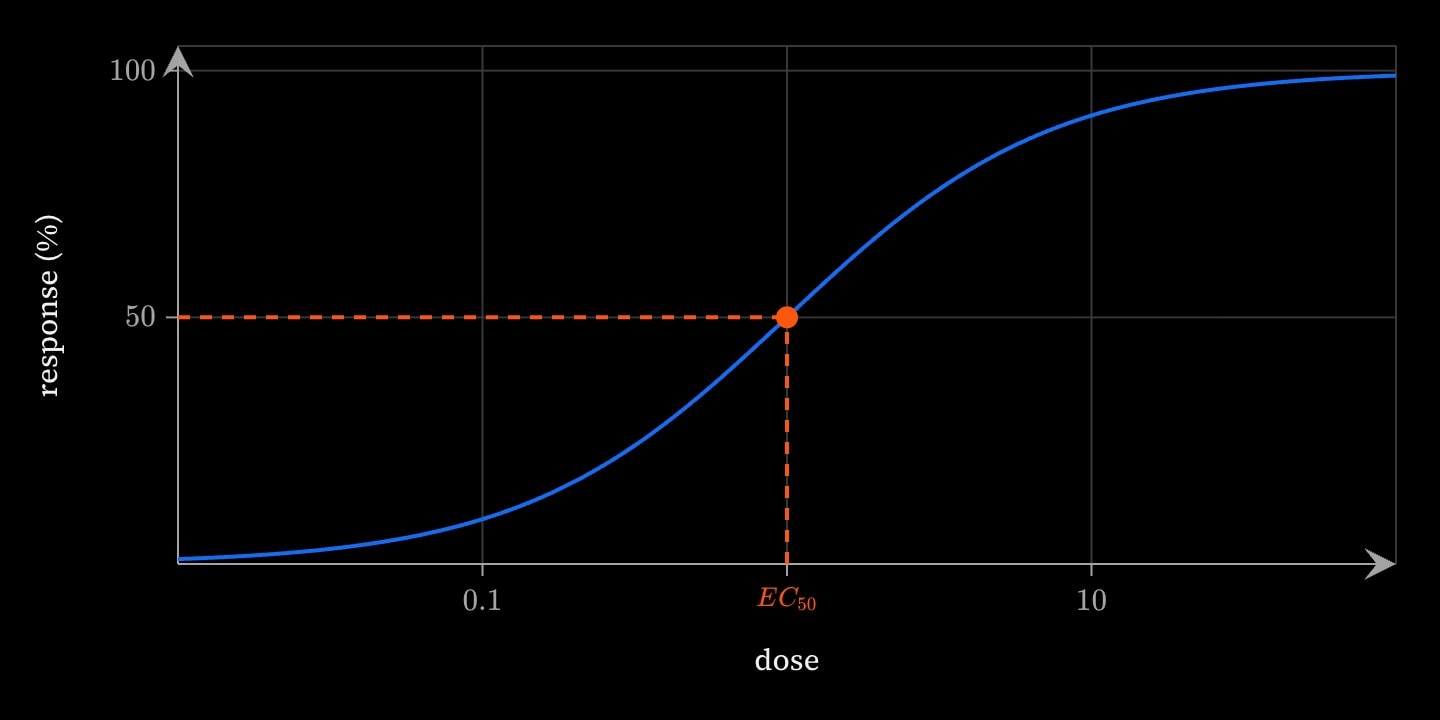
purplebiology.dose-responseA dose–response curve, the four-parameter logistic , with marked halfway between the floor and the ceiling. Drawn on a log dose axis — give the graph
x scale: log, where the curve is the symmetric sigmoid it is taught as.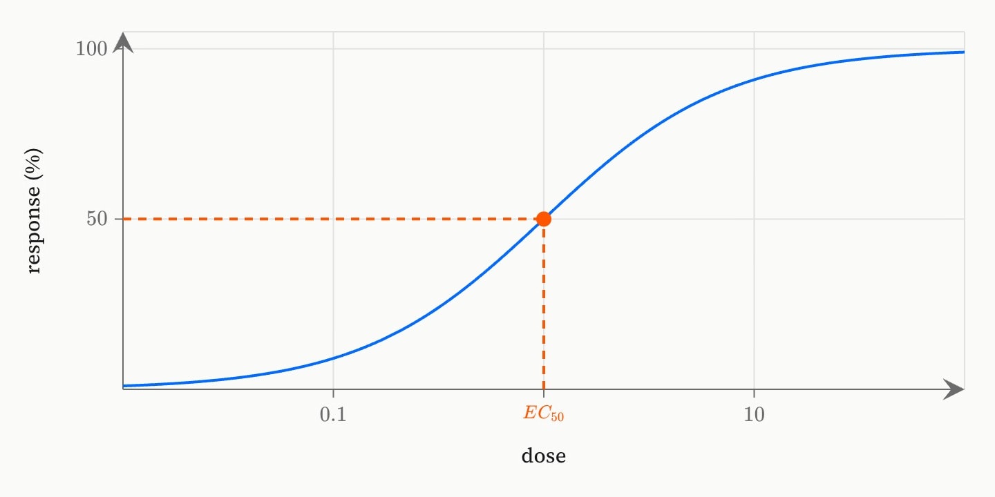
ec50The dose at half the maximum response, .
Default
1slopeThe Hill slope: how steeply the response rises through .
Default
1bottomThe response with no drug, the curve's floor.
Default
0topThe maximum response, the curve's ceiling.
Default
100fromThe lowest dose drawn. Above zero, since the dose axis is logarithmic.
Default
0.01toThe highest dose drawn.
Default
100labelThe curve's label.
inlineDefault
ec50-labelThe label on the dose axis at .
inlineDefault
$EC_{50}$colourThe curve's colour.
bluelight-bluedark-blueredlight-reddark-redorangelight-orangedark-orangeyellowlight-yellowdark-yellowteallight-tealdark-tealgreenlight-greendark-greenpinklight-pinkdark-pinkpurplelight-purpledark-purplegreylight-greydark-greyneutralhex(…)rgb(…)Default
bluemarker-colourThe half-maximum point and its dashed segments' colour.
bluelight-bluedark-blueredlight-reddark-redorangelight-orangedark-orangeyellowlight-yellowdark-yellowteallight-tealdark-tealgreenlight-greendark-greenpinklight-pinkdark-pinkpurplelight-purpledark-purplegreylight-greydark-greyneutralhex(…)rgb(…)Default
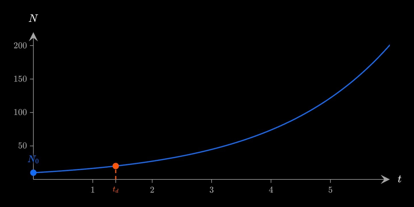
orangebiology.exponential-growthExponential growth , with the starting population marked and the doubling time dropped to the time axis.
r above zero.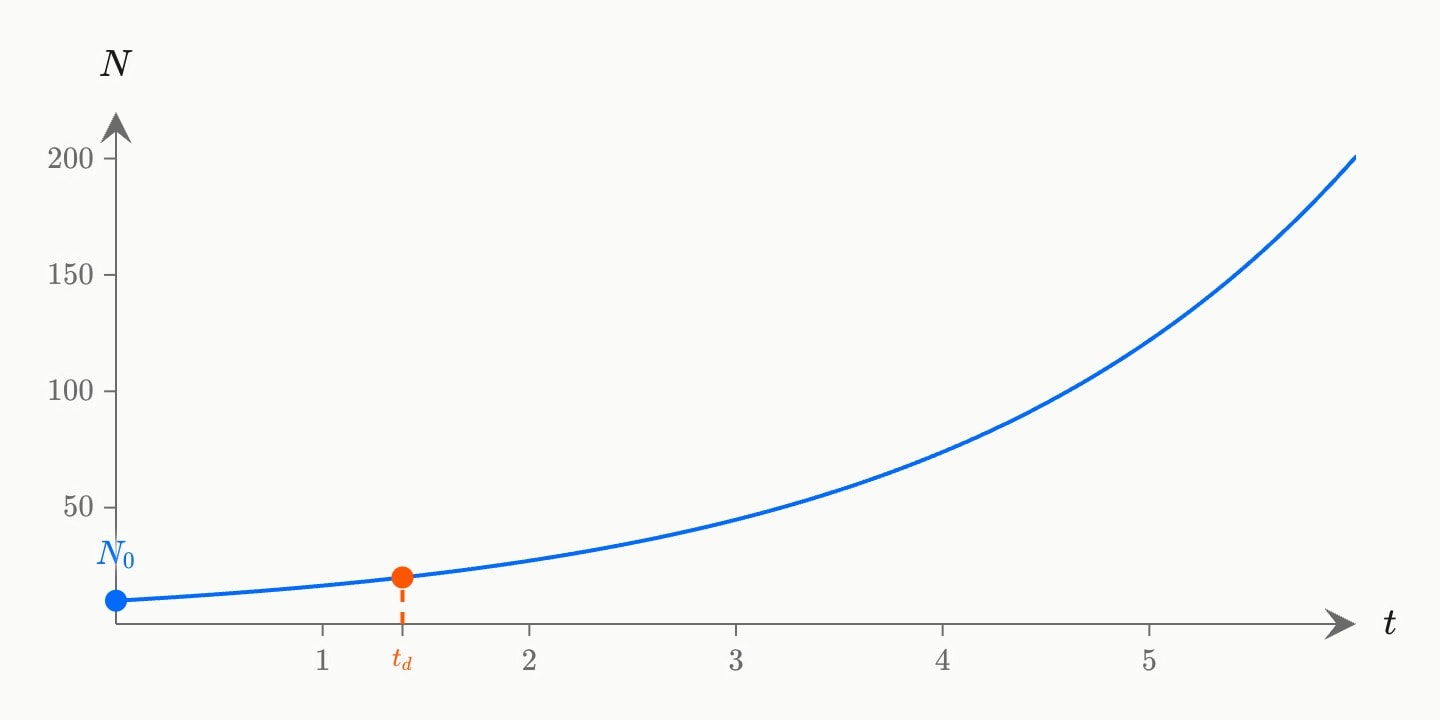
rThe growth rate per unit time, .
Default
0.5n0The population at time zero, .
Default
10tmaxThe time the curve is drawn out to.
Default
6labelThe curve's label.
inlineDefault
n0-labelThe starting population's label.
inlineDefault
$N_0$doubling-labelThe label on the time axis at the doubling time.
inlineDefault
$t_d$colourThe curve and the starting population's colour.
bluelight-bluedark-blueredlight-reddark-redorangelight-orangedark-orangeyellowlight-yellowdark-yellowteallight-tealdark-tealgreenlight-greendark-greenpinklight-pinkdark-pinkpurplelight-purpledark-purplegreylight-greydark-greyneutralhex(…)rgb(…)Default
bluemarker-colourThe doubled population's point and dashed segment's colour.
bluelight-bluedark-blueredlight-reddark-redorangelight-orangedark-orangeyellowlight-yellowdark-yellowteallight-tealdark-tealgreenlight-greendark-greenpinklight-pinkdark-pinkpurplelight-purpledark-purplegreylight-greydark-greyneutralhex(…)rgb(…)Default
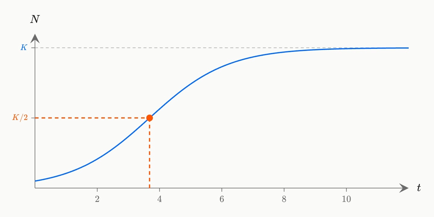
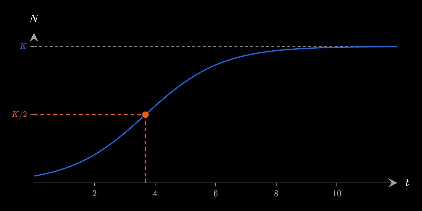
orangebiology.logistic-growthLogistic growth : the population levelling off at the carrying capacity , ruled across the plot, with the inflection at — where growth is fastest — dropped to both axes. The inflection comes at , after the start only when is below .
rThe intrinsic growth rate, .
Default
0.8kThe carrying capacity, .
Default
100n0The population at time zero, , below .
Default
5tmaxThe time the curve is drawn out to.
Default
12labelThe curve's label.
inlineDefault
k-labelThe label on the ruled line at the carrying capacity.
inlineDefault
$K$half-labelThe label on the population axis at the inflection.
inlineDefault
$K/2$colourThe curve and the carrying capacity's colour.
bluelight-bluedark-blueredlight-reddark-redorangelight-orangedark-orangeyellowlight-yellowdark-yellowteallight-tealdark-tealgreenlight-greendark-greenpinklight-pinkdark-pinkpurplelight-purpledark-purplegreylight-greydark-greyneutralhex(…)rgb(…)Default
bluemarker-colourThe inflection point and its dashed segments' colour.
bluelight-bluedark-blueredlight-reddark-redorangelight-orangedark-orangeyellowlight-yellowdark-yellowteallight-tealdark-tealgreenlight-greendark-greenpinklight-pinkdark-pinkpurplelight-purpledark-purplegreylight-greydark-greyneutralhex(…)rgb(…)Default
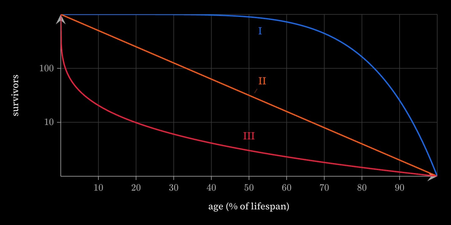
orangebiology.survivorshipThe three survivorship curves: survivors from a cohort against age, on a log survivors axis. Type I holds on until old age (large mammals), type II loses the same fraction at every age and is straight on the log axis (many birds), and type III loses most of the cohort young (fish, plants). All three start at the whole cohort and reach one survivor at
lifespan. Give the graph y scale: log and a y domain from 1 to the cohort.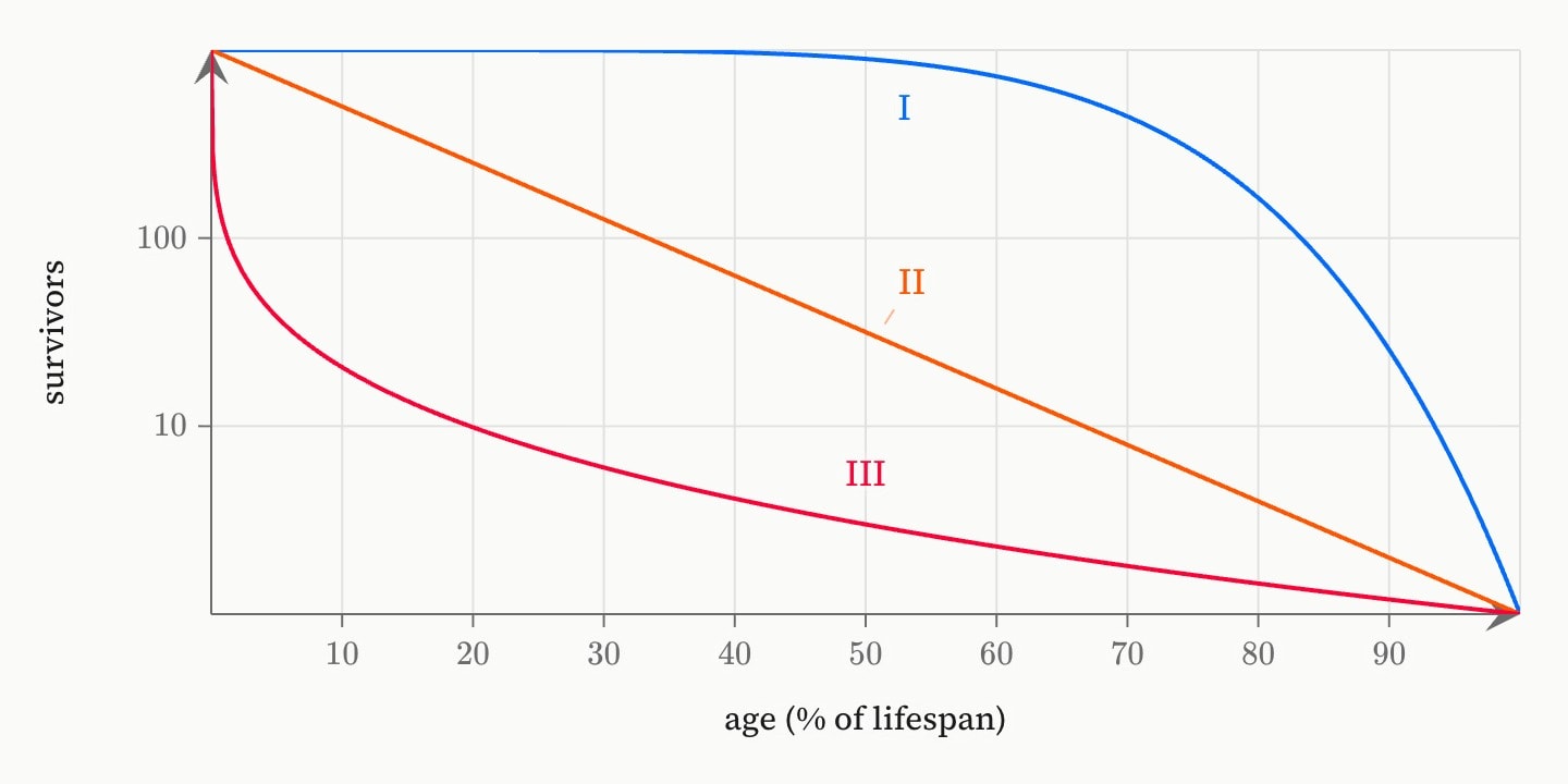
lifespanThe age at which one survivor is left.
Default
100cohortHow many the cohort starts with.
Default
1000type-1-labelThe type I curve's label.
inlineDefault
Itype-2-labelThe type II curve's label.
inlineDefault
IItype-3-labelThe type III curve's label.
inlineDefault
IIItype-1-colourThe type I curve's colour.
bluelight-bluedark-blueredlight-reddark-redorangelight-orangedark-orangeyellowlight-yellowdark-yellowteallight-tealdark-tealgreenlight-greendark-greenpinklight-pinkdark-pinkpurplelight-purpledark-purplegreylight-greydark-greyneutralhex(…)rgb(…)Default
bluetype-2-colourThe type II curve's colour.
bluelight-bluedark-blueredlight-reddark-redorangelight-orangedark-orangeyellowlight-yellowdark-yellowteallight-tealdark-tealgreenlight-greendark-greenpinklight-pinkdark-pinkpurplelight-purpledark-purplegreylight-greydark-greyneutralhex(…)rgb(…)Default
orangetype-3-colourThe type III curve's colour.
bluelight-bluedark-blueredlight-reddark-redorangelight-orangedark-orangeyellowlight-yellowdark-yellowteallight-tealdark-tealgreenlight-greendark-greenpinklight-pinkdark-pinkpurplelight-purpledark-purplegreylight-greydark-greyneutralhex(…)rgb(…)Default
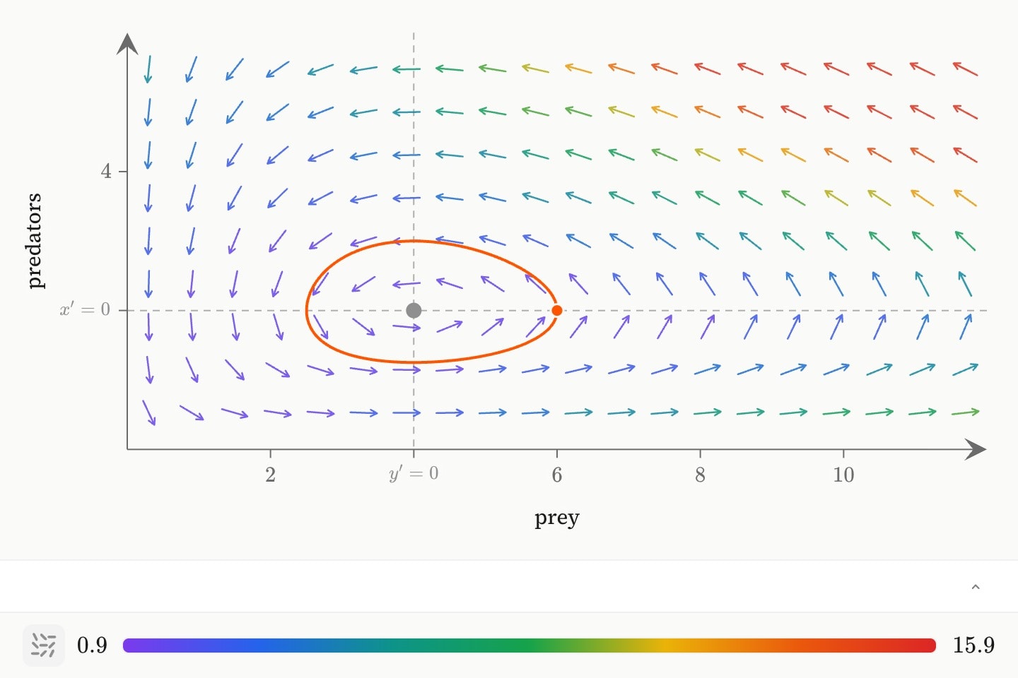
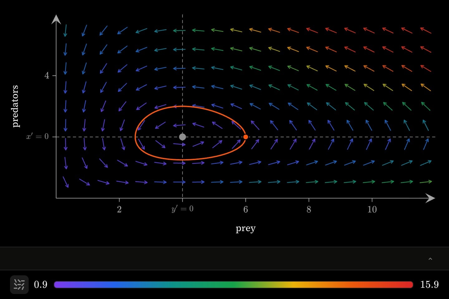
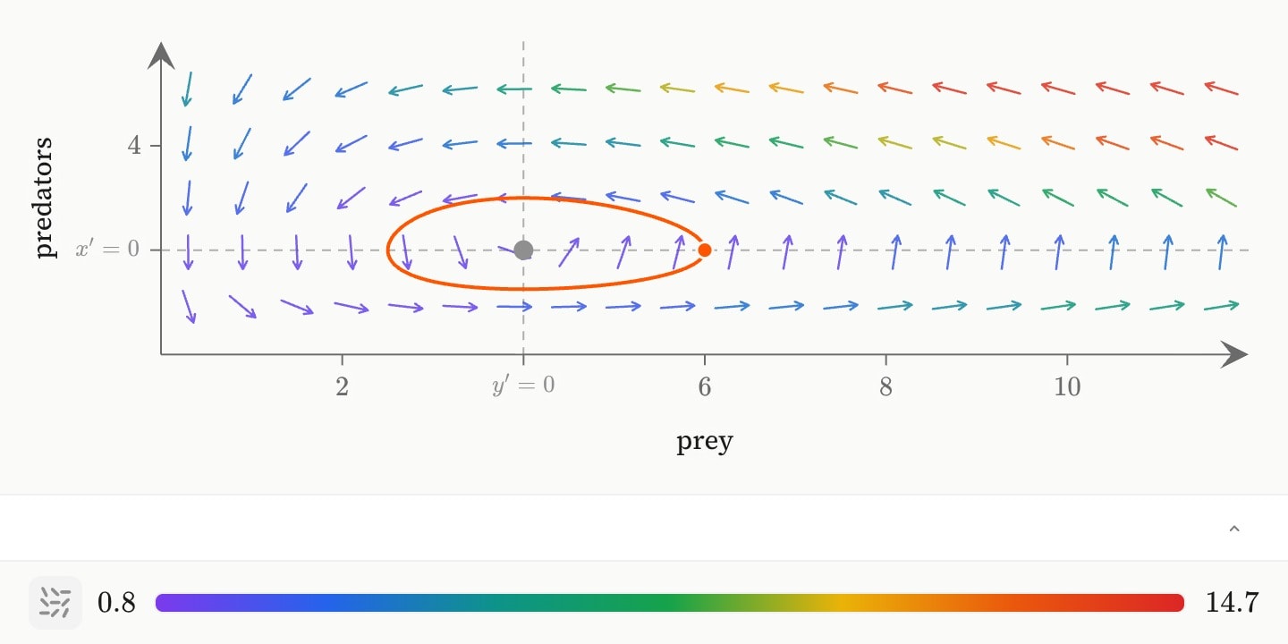
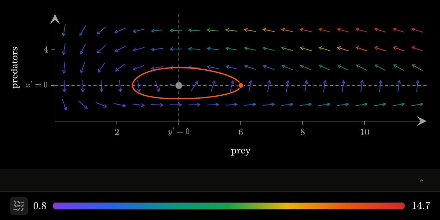
redbiology.predator-prey-phaseThe Lotka–Volterra predator–prey system in its phase plane, prey across and predators up: , . The field's arrows show the flow, a solution circles the equilibrium from a seed the reader can drag, and the two nullclines are ruled across the plot, meeting at the equilibrium .
alphaThe prey's growth rate with no predators, .
Default
1betaThe rate predators take prey, .
Default
0.5deltaThe rate prey eaten turns into predators, .
Default
0.25gammaThe predators' death rate with no prey, .
Default
1preyThe prey population the solution starts from.
Default
6predatorsThe predator population the solution starts from.
Default
2prey-nullcline-labelThe label on the prey's nullcline, the ruled line where .
inlineDefault
$x' = 0$predator-nullcline-labelThe label on the predators' nullcline, the ruled line where .
inlineDefault
$y' = 0$colourThe solution and its seed's colour.
bluelight-bluedark-blueredlight-reddark-redorangelight-orangedark-orangeyellowlight-yellowdark-yellowteallight-tealdark-tealgreenlight-greendark-greenpinklight-pinkdark-pinkpurplelight-purpledark-purplegreylight-greydark-greyneutralhex(…)rgb(…)Default
orangenullcline-colourThe nullclines and the equilibrium's colour.
bluelight-bluedark-blueredlight-reddark-redorangelight-orangedark-orangeyellowlight-yellowdark-yellowteallight-tealdark-tealgreenlight-greendark-greenpinklight-pinkdark-pinkpurplelight-purpledark-purplegreylight-greydark-greyneutralhex(…)rgb(…)Default
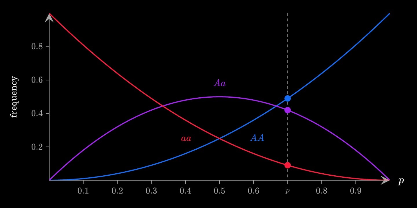
greybiology.hardy-weinbergGenotype frequencies under Hardy–Weinberg equilibrium against the frequency of allele : for , for and for , with . The heterozygotes peak at a half where .
marked rules a line at at and marks the three frequencies on it.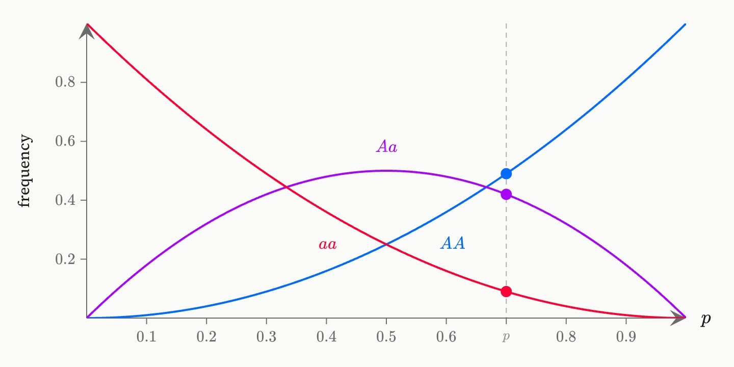
atThe frequency of the line is ruled at.
Default
0.7markedRule a line at
at and mark the three genotype frequencies on it.boolDefault
trueat-labelThe label on the ruled line.
inlineDefault
$p$dominant-labelThe curve's label.
inlineDefault
$AA$heterozygote-labelThe curve's label.
inlineDefault
$Aa$recessive-labelThe curve's label.
inlineDefault
$aa$dominant-colourThe curve and point's colour.
bluelight-bluedark-blueredlight-reddark-redorangelight-orangedark-orangeyellowlight-yellowdark-yellowteallight-tealdark-tealgreenlight-greendark-greenpinklight-pinkdark-pinkpurplelight-purpledark-purplegreylight-greydark-greyneutralhex(…)rgb(…)Default
blueheterozygote-colourThe curve and point's colour.
bluelight-bluedark-blueredlight-reddark-redorangelight-orangedark-orangeyellowlight-yellowdark-yellowteallight-tealdark-tealgreenlight-greendark-greenpinklight-pinkdark-pinkpurplelight-purpledark-purplegreylight-greydark-greyneutralhex(…)rgb(…)Default
purplerecessive-colourThe curve and point's colour.
bluelight-bluedark-blueredlight-reddark-redorangelight-orangedark-orangeyellowlight-yellowdark-yellowteallight-tealdark-tealgreenlight-greendark-greenpinklight-pinkdark-pinkpurplelight-purpledark-purplegreylight-greydark-greyneutralhex(…)rgb(…)Default
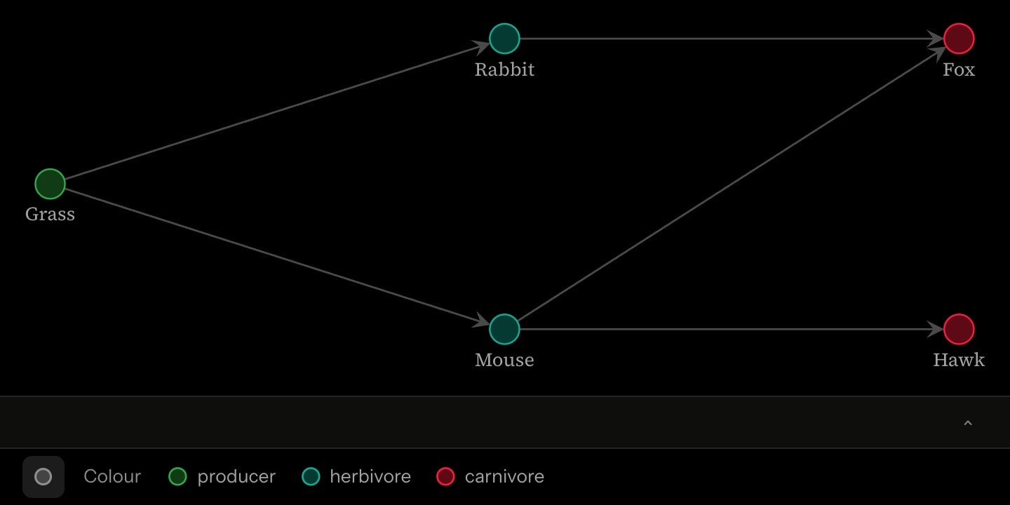
redbiology.food-webA food web: write each species as a
vertex whose group is what it eats — producer, herbivore, omnivore, carnivore, decomposer — and each feeding link as an edge from the food to the eater, the way energy flows. The web is laid out in trophic levels running left to right, producers first, and each group takes its colour in the key. A group not in that list is dealt a colour of its own.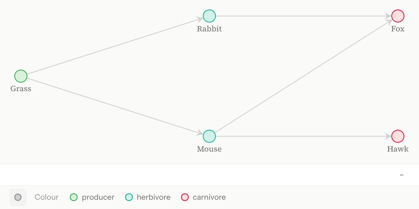
titleA title set above the web.
inlineDefault
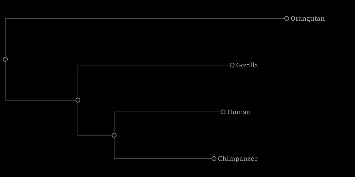
biology.phylogenyA phylogenetic tree: write each taxon and each ancestor as a
vertex, the root first, and each branch as an edge from ancestor to descendant. The tree runs left to right with square branches, each name set past its tip. lengths reads each edge's weight as its branch length, so the tree is a phylogram; off, every branch is one long and the tree is a cladogram, which shows only the branching order. Give the ancestors a small size, so the branches meet at a point rather than a disc.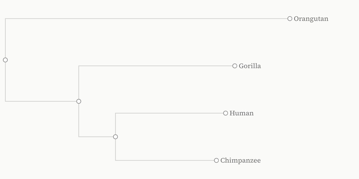
lengthsRead each edge's
weight as its branch length.boolDefault
truetitleA title set above the tree.
inlineDefault
#Datasets
#biology.lynx-hareSnowshoe hare and Canada lynx pelts traded to the Hudson's Bay Company, 1900–1920, in thousands — the predator–prey cycle every ecology course shows, the lynx peaking a year or two after the hares.
year, hare, lynx.Reach a column as
#biology.lynx-hare.<column>.#biology.mendelMendel's second-generation pea counts (1866), one row per trait: each trait's dominant and recessive forms and how many plants showed each, every trait near three to one.
trait, dominant, recessive, dominant-count, recessive-count.Reach a column as
#biology.mendel.<column>.